Introduction to Bayesian Regression

Standard regression finds a single "best" set of weights and makes predictions using only those weights. Bayesian regression takes a fundamentally different approach: instead of finding one answer, it maintains a distribution over all possible weight vectors, updating this distribution as data is observed. This naturally produces uncertainty estimates alongside predictions — telling us not just what the model predicts, but how confident it is.

This post covers the full Bayesian regression pipeline: Bayes' rule, Gaussian priors, the likelihood function, maximum likelihood estimation, closed-form posterior computation, and predictive distributions with uncertainty bands.

1. The Setup: Forrester Function

We use the Forrester function as our benchmark, with only 3 training points to make the uncertainty clearly visible:

def forrester_function(x):
    return (6*x - 2)**2 * np.sin(12*x - 4)

x = np.linspace(0, 1, 101)[:, np.newaxis]
t = forrester_function(x)

x_train = np.array([[0.2], [0.45], [0.9]])
t_train = forrester_function(x_train)

With only 3 data points and a complex underlying function, there is substantial ambiguity about the true relationship. This is exactly where Bayesian methods shine — they quantify this ambiguity explicitly.

2. Bayes' Rule

The core of Bayesian inference is Bayes' rule, which relates four quantities:

p(w|D) = p(D|w) · p(w) / p(D)

• Prior p(w): What we believe about the weights before seeing any data.
• Likelihood p(D|w): How probable the observed data is, given a specific weight vector.
• Posterior p(w|D): Our updated beliefs about the weights after seeing the data.
• Evidence p(D): A normalizing constant that ensures the posterior integrates to 1.

The posterior combines prior knowledge with evidence from data. With more data, the posterior becomes increasingly concentrated around the true weights, and the prior's influence diminishes.

3. The Gaussian Prior

We place a multivariate Gaussian prior over the weight vector:

p(w) = N(w; m₀, S₀)

where m₀ is the prior mean and S₀ is the prior covariance matrix. An uninformative prior uses m₀ = 0 and a large covariance S₀ = s²I, expressing that we have no strong prior beliefs about the weights.

def gaussian_pdf(x, m, S):
    D = len(x)
    det_S = np.linalg.det(S)
    inv_S = np.linalg.inv(S)
    norm = 1. / np.sqrt((2 * np.pi) ** D * det_S)
    return norm * np.exp(-0.5 * (x - m).T @ inv_S @ (x - m))

Sampling from the Prior

To understand what the prior implies, we can sample weight vectors from it and plot the corresponding prediction functions:

m = np.zeros((2, 1))
S = 10 * np.eye(2)

n_samples = 10
w_samples = np.random.multivariate_normal(m[:, 0], S, n_samples)

# Each sample produces a different line
y = x_f @ w_samples.T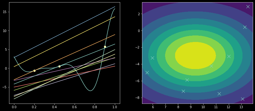

The left panel shows the function space view: 10 linear functions sampled from the prior, each corresponding to a different weight vector. The right panel shows the weight space view: a 2D Gaussian contour centered at the origin, with the sampled weight vectors marked. The correspondence between these two views is a central insight of Bayesian regression.

4. The Likelihood Function

The likelihood measures how well a particular weight vector explains the observed data. Under an additive Gaussian noise model:

t = y(x, w) + ε,   ε ~ N(0, σ_e²)

For i.i.d. observations, the joint likelihood is the product of individual likelihoods:

p(t|x, w) = ∏_i N(t_i; y(x_i, w), σ_e²)

In practice, we work with the log-likelihood to avoid numerical underflow from multiplying many small probabilities:

ln p(t|x, w) = -n/2 ln(σ_e²) - n/2 ln(2π) - 1/(2σ_e²) ∑_i (t_i - y_i)²

The last term is simply the sum-of-squared-errors (SSE). This reveals that maximizing the likelihood is equivalent to minimizing the MSE — standard regression is a special case of Bayesian inference.

5. Maximum Likelihood Estimation

The Maximum Likelihood Estimate (MLE) is the weight vector that maximizes the likelihood function. For linear regression, this is the familiar least-squares solution:

w_mle = np.linalg.inv(x_f_train.T @ x_f_train) @ x_f_train.T @ t_train

The MLE gives a single point estimate with no uncertainty. Bayesian regression goes further by computing the full posterior distribution.

6. Monte Carlo Predictive Uncertainty

Before deriving the closed-form posterior, we can approximate the predictive distribution by sampling. Drawing many weight vectors from the prior and computing predictions for each gives us a distribution over outputs:

n_samples = 5000
w_samples = np.random.multivariate_normal(m[:, 0], S, n_samples)
y_samples = w_samples @ x_f.T

y_mean = np.mean(y_samples, axis=0)
y_std = np.std(y_samples, axis=0)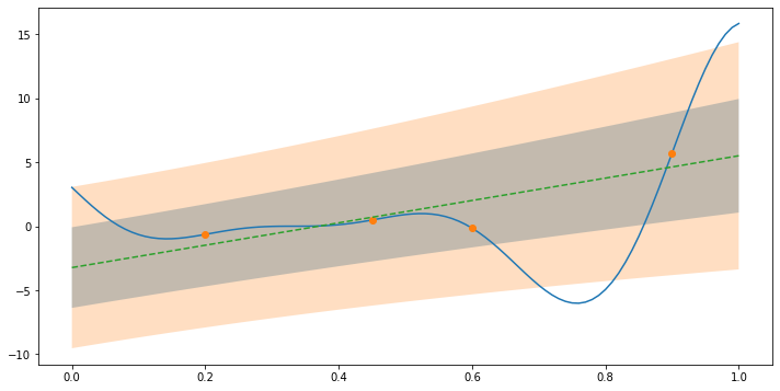

The shaded bands show regions where the model predicts the function might lie. With only a prior (no data incorporated yet), the uncertainty is broad and nearly uniform across the input range.

7. Closed-Form Posterior (Conjugate Update)

When both the prior and likelihood are Gaussian, the posterior is also Gaussian — this is the conjugate prior property. The posterior parameters have a beautiful closed-form solution:

Posterior covariance:

S_N = (S₀^-1 + θ_x^T Σ_e^-1 θ_x)^-1

Posterior mean:

m_N = S_N(S₀^-1 m₀ + θ_x^T Σ_e^-1 t)

Predictive distribution:

p(t̂|x̂, x, t) = N(t̂; m_N^Tθ_x̂, θ_x̂ S_N θ_x̂^T)

# Bayesian inference in 4 lines
S_0_inv = np.linalg.inv(S_0)
Sigma_e_inv = np.linalg.inv(sigma_e**2 * np.eye(N))

S_N = np.linalg.inv(S_0_inv + x_f_train.T @ Sigma_e_inv @ x_f_train)
m_N = S_N @ (S_0_inv @ m_0 + x_f_train.T @ Sigma_e_inv @ t_train)

8. The Complete Picture: Prior, Likelihood, Posterior

The culminating visualization shows all three components of Bayes' rule in both weight space and function space:

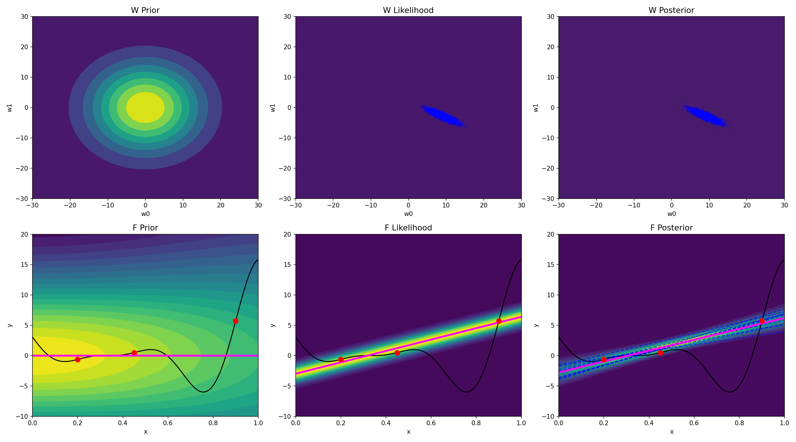
Top row (Weight Space):

• Prior: A broad 2D Gaussian centered at zero. All weight vectors are roughly equally plausible.
• Likelihood: The data constrains which weight vectors are plausible. The likelihood is concentrated along a narrow band in weight space.
• Posterior: The product of prior and likelihood. A sharply peaked distribution centered near the weight values that both explain the data and are consistent with the prior.

Bottom row (Function Space):

• Prior: Broad contour showing high uncertainty everywhere. The mean prediction (magenta) is a flat line at zero.
• Likelihood: The MLE prediction (magenta line) passes through the training points. The contour shows the likelihood of observations at each point.
• Posterior: Uncertainty is narrowest near the training points (where we have evidence) and widest far from them (where we are less certain). Sampled functions (blue dashed lines) all pass near the training points but diverge elsewhere.

This is the key insight of Bayesian regression: uncertainty is heterogeneous. The model is confident where it has data and honestly uncertain where it does not.

9. Key Takeaways

1. Bayesian regression quantifies uncertainty: Instead of a single prediction, you get a distribution. The width of the predictive distribution tells you how much to trust the prediction.
2. The prior encodes domain knowledge: An uninformative prior lets the data speak for itself. An informative prior can incorporate expert knowledge, accelerating learning with limited data.
3. Conjugate Gaussians yield closed-form solutions: When both prior and likelihood are Gaussian, the posterior is Gaussian too. No sampling or approximation needed — just matrix algebra.
4. MLE is a special case: Maximizing the likelihood is equivalent to minimizing MSE. Bayesian regression reduces to standard regression when the prior is infinitely broad.
5. Weight space and function space are dual views: Every distribution over weights implies a distribution over functions, and vice versa. Understanding both views gives deeper insight into model behavior.