Convolutional Neural Networks (CNNs) for Image Classification
Convolutional Neural Networks are the backbone of modern computer vision. Unlike fully connected networks that treat each pixel independently, CNNs exploit the spatial structure of images through local connectivity and weight sharing, making them far more efficient and effective for visual recognition tasks.
In this post, we walk through the complete pipeline of building, training, and evaluating vanilla CNN architectures for image classification on the Fashion MNIST dataset. We systematically compare how architectural choices — padding strategy, network depth, and kernel size — affect both model capacity and generalization performance.
1. The Dataset: Fashion MNIST
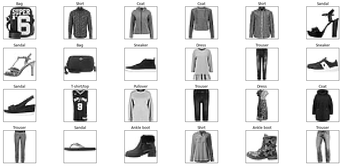
Fashion MNIST is a drop-in replacement for the classic MNIST handwritten digits dataset, proposed by Zalando Research. It contains 70,000 grayscale images of size 28×28, distributed across 10 clothing categories: T-shirt/top, Trouser, Pullover, Dress, Coat, Sandal, Shirt, Sneaker, Bag, and Ankle boot.
The dataset provides a more challenging benchmark than MNIST digits while maintaining the same convenient format. We split the data into three subsets:
- Training set: 54,000 images (90% of the original training data)
- Validation set: 6,000 images (10% held out from training)
- Test set: 10,000 images (untouched during training)
(x_train, y_train), (x_test, y_test) = fashion_mnist.load_data()

# Hold out 10% as validation set
n_val = int(0.1 * len(x_train))

x_val = x_train[:n_val]
x_train = x_train[n_val:]

y_val = y_train[:n_val]
y_train = y_train[n_val:]
Below is a sample grid from the training set, illustrating the diversity of items within each class:
2. Data Preprocessing
Raw pixel values range from 0 to 255 as unsigned 8-bit integers. Before feeding images into a neural network, we apply two essential transformations:
- Dimension expansion: CNNs expect a channel dimension. We reshape each image from
(28, 28)to(28, 28, 1), explicitly encoding the single grayscale channel. - Min-Max normalization: We scale pixel values to the [0, 1] range by dividing by 255. This keeps gradient magnitudes well-behaved and accelerates convergence.
# (#, 28, 28) => (#, 28, 28, 1)
# uint8 => float32
# [0, 255] => [0, 1]
x_train = np.expand_dims(x_train, axis=-1).astype("float32") / 255.0
x_val   = np.expand_dims(x_val, axis=-1).astype("float32") / 255.0
x_test  = np.expand_dims(x_test, axis=-1).astype("float32") / 255.0
An alternative normalization strategy is standardization (zero mean, unit variance), computed as x_std = (x − μ) / σ. Min-Max is generally preferred for image data because pixel intensities have a natural bounded range, but standardization can be advantageous when working with pre-trained models that expect standardized inputs.
3. Custom Data Generator
For production-grade training, especially when datasets are too large to fit in memory, we implement a custom data generator by subclassing keras.utils.Sequence. This provides several advantages:
- Memory efficiency: Only one batch resides in memory at any given time.
- Shuffling: Data is reshuffled at the end of each epoch, preventing the network from memorizing batch order.
- Multiprocessing compatibility: The Sequence interface guarantees thread-safe batch generation.
class DataGenerator(keras.utils.Sequence):
    def __init__(self, batch_size, data, labels, shuffle=True):
        self.batch_size = batch_size
        self.data = data
        self.labels = labels
        self.shuffle = shuffle

    def on_epoch_end(self):
        if self.shuffle:
            self.data, self.labels = shuffle(self.data, self.labels)

    def __len__(self):
        return self.data.shape[0] // self.batch_size

    def __getitem__(self, idx):
        i = idx * self.batch_size
        batch_images = self.data[i : i + self.batch_size]
        batch_labels = self.labels[i : i + self.batch_size]
        return batch_images, batch_labels
We instantiate generators for both training and validation with a batch size of 128:
batch_size = 128
data_gen_train = DataGenerator(batch_size=batch_size, data=x_train, labels=y_train)
data_gen_val   = DataGenerator(batch_size=batch_size, data=x_val, labels=y_val)
4. CNN Architecture Design
A vanilla CNN for classification follows a well-established pattern: a series of convolutional blocks (convolution + pooling) that extract increasingly abstract features, followed by fully connected layers that map those features to class probabilities.
Each convolutional block in our design consists of:
- A
Conv2Dlayer with 3×3 kernels and ReLU activation - A
MaxPooling2Dlayer with 2×2 pool size, halving the spatial dimensions
Sequential vs. Functional API
Keras offers two paradigms for model construction. The Sequential API is concise and intuitive for linear stacks of layers — each layer has exactly one input tensor and one output tensor. The Functional API is more expressive, supporting architectures with shared layers, multiple inputs/outputs, and skip connections.
Sequential API
def get_model(filters, n_classes, k=3, name="my_model", padding="valid"):
    model = Sequential(name=name)
    # First convolutional block
    model.add(Conv2D(filters[0], (k, k), input_shape=(28, 28, 1),
                     activation="relu", padding=padding))
    model.add(MaxPooling2D(2, 2))

    # Additional convolutional blocks
    for n in filters[1:]:
        model.add(Conv2D(n, (k, k), activation="relu", padding=padding))
        model.add(MaxPooling2D(2, 2))

    # Classification head
    model.add(Flatten())
    model.add(Dense(100, activation="relu"))
    model.add(Dense(n_classes, activation="softmax"))

    model.compile(optimizer=Adam(learning_rate=0.001),
                  loss=tf.keras.losses.SparseCategoricalCrossentropy(),
                  metrics=['accuracy'])
    return model
Functional API
def get_model_funct(filters, n_classes, k=3, name="my_model", padding="valid"):
    input_layer = Input(shape=(28, 28, 1))
    x = Conv2D(filters[0], (k, k), activation="relu", padding=padding)(input_layer)
    x = MaxPooling2D(2, 2)(x)

    for n in filters[1:]:
        x = Conv2D(n, (k, k), activation="relu", padding=padding)(x)
        x = MaxPooling2D(2, 2)(x)

    x = Flatten()(x)
    x = Dense(100, activation="relu")(x)
    output_layer = Dense(n_classes, activation="softmax")(x)

    model = Model(inputs=input_layer, outputs=output_layer, name=name)
    model.compile(optimizer=Adam(learning_rate=0.001),
                  loss=tf.keras.losses.SparseCategoricalCrossentropy(),
                  metrics=['accuracy'])
    return model
5. Experiment 1: Padding and Depth
We instantiate three model variants to study the effect of padding and network depth:
- Vanilla CNN 1 — Single conv block,
validpadding (no padding) - Vanilla CNN 2 — Single conv block,
samepadding (zero-padded borders) - Vanilla CNN 3 — Two conv blocks [32, 64 filters],
samepadding
model_cnn_vanilla_1 = get_model(filters=[32],
                                n_classes=n_classes,
                                name="Vanilla_CNN_1",
                                padding="valid")

model_cnn_vanilla_2 = get_model(filters=[32],
                                n_classes=n_classes,
                                name="Vanilla_CNN_2_Padding",
                                padding="same")

model_cnn_vanilla_3 = get_model_funct(filters=[32, 64],
                                      n_classes=n_classes,
                                      name="Vanilla_CNN_3_Padding_Deep",
                                      padding="same")
Architecture Summaries
Examining the parameter counts reveals a counterintuitive insight:
- CNN 1 (valid padding, 1 block): 542,230 parameters
- CNN 2 (same padding, 1 block): 628,630 parameters
- CNN 3 (same padding, 2 blocks): 333,526 parameters
The deeper network (CNN 3) has fewer parameters than the shallower ones. This is because the second pooling layer further reduces the spatial dimensions before flattening, dramatically shrinking the dense layer input. With valid padding, a 3×3 convolution on a 28×28 input yields 26×26 output; after pooling, that becomes 13×13 = 169 spatial positions × 32 filters = 5,408 features going into the dense layer. With same padding and two blocks, the spatial dimensions reduce to 7×7, yielding only 3,136 features despite using 64 filters in the second block.
This illustrates a fundamental principle: deeper architectures with progressive spatial reduction are more parameter-efficient than wide, shallow ones.
Training Configuration
All models are trained with the Adam optimizer (lr=0.001), sparse categorical cross-entropy loss, and two callbacks:
- ModelCheckpoint: Saves the best model weights based on validation accuracy.
- EarlyStopping: Halts training if no improvement is seen for 30 consecutive epochs, preventing wasted computation.
mode_autosave = ModelCheckpoint("model.h5",
                                mode="max",
                                save_best_only=True,
                                monitor="val_accuracy",
                                verbose=1)

early_stopping = EarlyStopping(patience=30, verbose=1, mode="auto")
Training Curves
The loss and accuracy curves across all three configurations reveal important patterns:
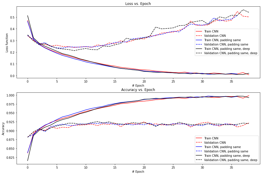
Key observations from the training curves:
- Overfitting in CNN 1: The red curves show a stark divergence between training and validation loss after epoch ~15. Training loss continues to decrease while validation loss rises — classic overfitting. This model memorizes the training data without learning generalizable patterns.
- Same padding helps regularization: CNN 2 (blue) shows less overfitting than CNN 1. By preserving border information, same padding provides the network with more spatial context.
- Depth improves generalization: CNN 3 (black) achieves the lowest validation loss despite having the fewest parameters. The deeper architecture extracts more hierarchical features, and the additional pooling acts as implicit regularization.
Evaluation Results
| Model | Train Loss | Val Loss | Test Loss | Train Acc | Val Acc | Test Acc |
|---|---|---|---|---|---|---|
| CNN 1 (valid) | 0.0342 | 0.3191 | 0.3122 | 99.01% | 92.36% | 91.89% |
| CNN 2 (same) | 0.0640 | 0.2593 | 0.2745 | 97.98% | 92.09% | 91.86% |
| CNN 3 (same, deep) | 0.0836 | 0.2220 | 0.2493 | 97.24% | 92.39% | 91.69% |
While CNN 1 achieves the highest training accuracy (99.01%), its validation and test losses are significantly worse. CNN 3, despite lower training accuracy, has the best validation loss (0.2220) and best test loss (0.2493). The gap between training and validation performance in CNN 1 (loss: 0.034 vs 0.319) is an order of magnitude, confirming severe overfitting. In CNN 3, this gap is much smaller (0.084 vs 0.222), indicating better generalization.
6. Experiment 2: Kernel Size
The receptive field of a convolutional kernel determines how much local context each neuron can observe. Larger kernels capture broader patterns but increase the parameter count and may capture noise. We compare four kernel sizes — 3×3, 5×5, 7×7, and 9×9 — using the same two-block [32, 64] architecture with same padding:
cnn_k_3 = get_model(filters=[32, 64], n_classes=n_classes, k=3, padding="same")
cnn_k_5 = get_model(filters=[32, 64], n_classes=n_classes, k=5, padding="same")
cnn_k_7 = get_model(filters=[32, 64], n_classes=n_classes, k=7, padding="same")
cnn_k_9 = get_model(filters=[32, 64], n_classes=n_classes, k=9, padding="same")
Training Curves
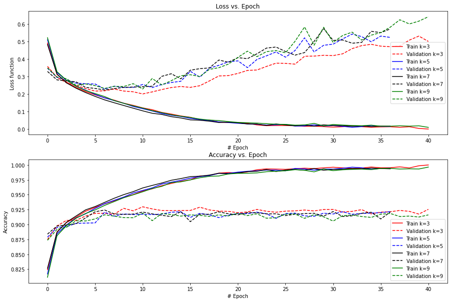
The training curves paint a clear picture:
- All models converge to near-perfect training accuracy, but their validation behavior diverges significantly.
- k=3 (red) shows the healthiest training dynamics — the validation loss remains the lowest and most stable throughout training.
- k=9 (green) exhibits the worst overfitting, with validation loss climbing sharply after epoch ~15 while training loss continues to drop.
- There is a clear monotonic relationship: larger kernels lead to greater overfitting on this dataset.
Evaluation Results
| Kernel | Train Loss | Val Loss | Test Loss | Train Acc | Val Acc | Test Acc |
|---|---|---|---|---|---|---|
| k = 3 | 0.0005 | 0.5013 | 0.5616 | 100.00% | 92.58% | 92.60% |
| k = 5 | 0.0062 | 0.5273 | 0.5817 | 99.80% | 92.19% | 91.90% |
| k = 7 | 0.0114 | 0.5811 | 0.6065 | 99.60% | 92.00% | 91.46% |
| k = 9 | 0.0092 | 0.6577 | 0.7331 | 99.65% | 91.51% | 91.00% |
The 3×3 kernel achieves the best generalization across all metrics. This aligns with a well-established principle in deep learning: stacking multiple small kernels is preferable to using a single large kernel. Two stacked 3×3 convolutions have the same effective receptive field as a single 5×5 convolution, but with fewer parameters and an additional non-linearity between them.
It is worth noting that on small images (28×28), a 9×9 kernel covers nearly a third of the spatial dimension in a single operation, which is excessive. The kernel captures too much global structure at once, losing the fine-grained local features that are critical for distinguishing between similar categories like Shirt vs. T-shirt or Coat vs. Pullover.
7. Key Takeaways
"More depth, smaller kernels, better generalization."
- Prefer
samepadding: It preserves spatial resolution and prevents border information loss. Withvalidpadding, each convolutional layer shrinks the feature map, compounding information loss at image boundaries. - Go deeper, not wider: Adding more convolutional blocks with progressive downsampling is more parameter-efficient than using a single block with many filters. Each pooling layer reduces the feature map size, keeping the dense layer compact.
- Use small kernels (3×3): They offer the best trade-off between local feature extraction and parameter efficiency. Larger receptive fields are better achieved by stacking layers rather than using large kernels.
- Monitor the train-validation gap: A large gap between training and validation performance is a reliable indicator of overfitting. Techniques like dropout, batch normalization, data augmentation, and weight decay can narrow this gap.
- Use callbacks wisely:
ModelCheckpointensures you always have access to the best-performing model, whileEarlyStoppingprevents wasted computation and further overfitting during extended training.
8. Best Practices for Reproducible Research
- Use relative paths for datasets and configuration files. Hardcoded absolute paths break portability and may expose sensitive directory structures.
- Use
.gitignoreto exclude large files (datasets, model weights, checkpoints) from version control. Share these via dedicated platforms like Zenodo or Google Drive. - Refactor your code: Extract hyperparameters into variables, remove stale comments, and follow PEP 8 conventions. Well-structured code is easier to debug, extend, and reproduce.
- Use git branches for experimental features. Merge into the main branch only after thorough testing. A naming convention like
feature/0002-add-new-modelskeeps branches organized.