CNN Training: Optimizers, Initializers & Data Augmentation

Training a Convolutional Neural Network is not just about designing the architecture — the choice of optimizer, weight initialization strategy, and data augmentation pipeline can dramatically affect whether the model converges, how fast it learns, and how well it generalizes. These are the hidden levers of deep learning that separate a model that barely trains from one that achieves state-of-the-art results.

In this post, we systematically compare different optimizers, initializers, and augmentation strategies using the UC Merced Land Use dataset — a challenging 21-class aerial image classification benchmark. Each experiment isolates a single variable while keeping everything else fixed, allowing us to draw clear conclusions.

1. The Dataset: UC Merced Land Use

The UC Merced Land Use dataset contains 2,100 aerial images (256×256 pixels, RGB) distributed evenly across 21 land use categories: agricultural, airplane, baseball diamond, beach, buildings, chaparral, dense residential, forest, freeway, golf course, harbor, intersection, medium residential, mobile home park, overpass, parking lot, river, runway, sparse residential, storage tanks, and tennis court.

We split the data using stratified sampling to ensure balanced class representation across splits:

• Training: 60% (1,260 images)
• Validation: 20% (420 images)
• Test: 20% (420 images)

# Stratified 80/20 split
x_train, x_test, y_train, y_test = train_test_split(
    df["path_image"].values, df["class_int"].values,
    train_size=0.8, test_size=0.2, stratify=df["class_int"].values)

# Further split training into 75/25 for train/validation
x_train, x_val, y_train, y_val = train_test_split(
    x_train, y_train,
    train_size=0.75, test_size=0.25, stratify=y_train)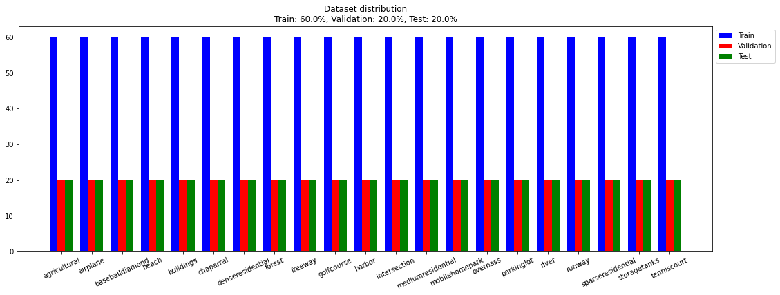

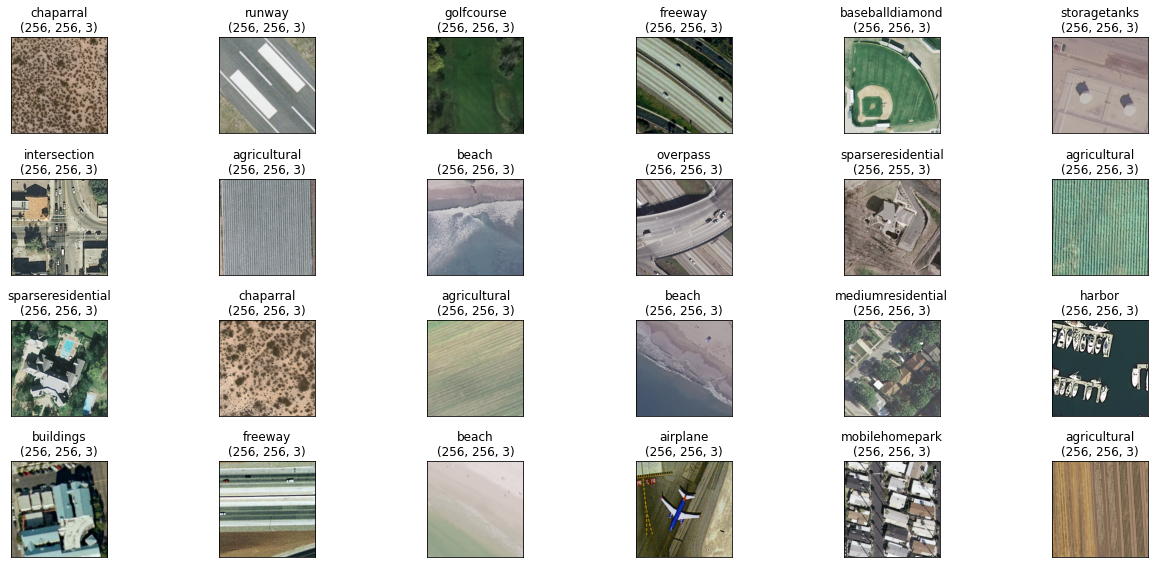
Unlike Fashion MNIST, this dataset presents real-world challenges: high intra-class variability (a parking lot can look very different depending on time of day and occupancy), subtle inter-class differences (medium vs. dense residential), and small dataset size (only 100 images per class).

2. Base Architecture

All experiments use an identical CNN backbone with 5 convolutional blocks [16, 32, 64, 128, 256 filters], each including:

• Conv2D with 3×3 kernels and ReLU activation
• BatchNormalization for stable gradients
• MaxPooling2D (2×2) for spatial downsampling
• Dropout (10%) for regularization

Followed by a fully connected classification head (100-unit dense layer + 21-class softmax output). Total: 1,318,413 parameters.

def get_model(filters, n_classes, optimizer, initializer,
              dropout=0.1, batch_norm=True, name="my_model"):
    model = Sequential(name=name)
    model.add(Conv2D(filters[0], (3,3), input_shape=(256,256,3),
                     activation="relu", kernel_initializer=initializer))
    if batch_norm: model.add(BatchNormalization())
    model.add(MaxPooling2D(2,2))
    if dropout: model.add(Dropout(dropout))

    for n in filters[1:]:
        model.add(Conv2D(n, (3,3), activation="relu",
                         kernel_initializer=initializer))
        if batch_norm: model.add(BatchNormalization())
        model.add(MaxPooling2D(2,2))
        if dropout: model.add(Dropout(dropout))

    model.add(Flatten())
    model.add(Dense(100, activation="relu", kernel_initializer=initializer))
    model.add(Dense(n_classes, activation="softmax"))

    model.compile(optimizer=optimizer,
                  loss="categorical_crossentropy",
                  metrics=['accuracy'])
    return model

3. Experiment 1: Optimizers

We compare four optimizers, all with learning rate 0.001 and Glorot Uniform initialization:

• SGD (Stochastic Gradient Descent): The classic optimizer. Uses only the current gradient, no momentum or adaptive learning rates.
• RMSprop: Divides the learning rate by a running average of recent gradient magnitudes. Adapts per-parameter.
• Adam: Combines momentum (first moment) with RMSprop-style adaptive rates (second moment). The most popular default choice.
• Adagrad: Adapts learning rate per parameter based on the historical sum of squared gradients. Naturally decays the learning rate over time.

model_sgd     = get_model(filters, n_classes, optimizer=SGD(lr=0.001),
                          initializer="glorot_uniform", name="CNN_SGD")
model_rmsprop = get_model(filters, n_classes, optimizer=RMSprop(lr=0.001),
                          initializer="glorot_uniform", name="CNN_RMSProp")
model_adam    = get_model(filters, n_classes, optimizer=Adam(lr=0.001),
                          initializer="glorot_uniform", name="CNN_Adam")
model_adagrad = get_model(filters, n_classes, optimizer=Adagrad(lr=0.001),
                          initializer="glorot_uniform", name="CNN_Adagrad")

Results

Optimizer	Train Loss	Val Loss	Test Loss	Train Acc	Val Acc	Test Acc
SGD	0.153	1.662	1.542	95.35%	55.77%	60.10%
RMSprop	3.332	13.164	13.363	74.68%	40.62%	41.83%
Adam	0.006	3.489	3.339	99.84%	64.90%	68.03%
Adagrad	0.120	1.681	1.769	96.15%	56.73%	58.41%

Key observations:

• Adam achieves the highest test accuracy (68.03%) with the lowest training loss, confirming its effectiveness as a general-purpose optimizer. However, its validation loss (3.489) is higher than SGD's (1.662), suggesting more aggressive overfitting.
• RMSprop struggles significantly on this dataset, with unstable training and the worst overall performance. Its sensitivity to hyperparameters is a known issue.
• SGD and Adagrad offer better loss calibration — their validation losses are much closer to training losses, indicating more stable generalization despite lower peak accuracy.
• All models show a massive generalization gap (95-99% train vs 40-68% test), which is expected on such a small dataset (only ~60 training images per class).

4. Experiment 2: Weight Initializers

Weight initialization determines the starting point for optimization. A poor initialization can prevent gradient flow entirely, making the model untrainable. We compare four strategies using the Adagrad optimizer:

• Zeros: All weights set to 0. Every neuron computes the same output — the symmetry is never broken.
• Ones: All weights set to 1. Activations explode through the network.
• Glorot Uniform (Xavier): Weights drawn from a uniform distribution scaled by fan-in and fan-out. Designed to maintain variance across layers.
• He Uniform: Similar to Glorot but scaled for ReLU activations, accounting for the fact that ReLU zeroes out half the outputs.

model_zeros  = get_model(filters, n_classes, optimizer=Adagrad(lr=0.001),
                         initializer="zeros", name="CNN_Zeros")
model_ones   = get_model(filters, n_classes, optimizer=Adagrad(lr=0.001),
                         initializer="ones", name="CNN_Ones")
model_glorot = get_model(filters, n_classes, optimizer=Adagrad(lr=0.001),
                         initializer="glorot_uniform", name="CNN_Glorot")
model_he     = get_model(filters, n_classes, optimizer=Adagrad(lr=0.001),
                         initializer="he_uniform", name="CNN_He")

Results

Initializer	Train Loss	Val Loss	Test Loss	Train Acc	Val Acc	Test Acc
Zeros	3.045	3.045	3.045	4.73%	4.33%	4.81%
Ones	9.006	17.430	12.105	12.26%	9.86%	11.06%
Glorot Uniform	0.156	1.771	1.768	95.35%	54.09%	55.53%
He Uniform	0.393	2.315	2.118	86.78%	45.19%	48.08%

The results are dramatic:

• Zeros initialization completely fails (4.73% train accuracy = random chance for 21 classes). With all weights at zero, every neuron computes the same gradient, and the symmetry is never broken. The network is essentially dead.
• Ones initialization barely trains (12.26%). Uniform positive weights cause activations to explode, producing unstable and poorly calibrated outputs.
• Glorot Uniform wins decisively (55.53% test accuracy). By scaling initial weights according to layer size, it maintains stable gradient flow throughout the network.
• He Uniform performs reasonably (48.08%) but underperforms Glorot here, likely because BatchNormalization partially compensates for the initialization scale, reducing He's advantage for ReLU networks.

Initialization is not just a detail — it determines whether your network can learn at all. Zero and constant initializations create symmetric neurons that can never differentiate.

5. Experiment 3: Data Augmentation

With only 1,260 training images across 21 classes, overfitting is inevitable. Data augmentation artificially expands the training set by applying random geometric and photometric transformations to each sample during training. We use the Albumentations library:

from albumentations import (Blur, Compose, HorizontalFlip,
    RandomBrightnessContrast, RandomRotate90, VerticalFlip)

def augmentation():
    return Compose([
        HorizontalFlip(p=0.5),
        VerticalFlip(p=0.5),
        RandomRotate90(p=0.5),
        Blur(p=0.01, blur_limit=3),
        RandomBrightnessContrast(p=0.5),
    ], p=1)

For aerial images, horizontal/vertical flips and 90-degree rotations are especially natural augmentations since there is no canonical "up" orientation in satellite/aerial views. Below we see original images (left) alongside their augmented versions (right):

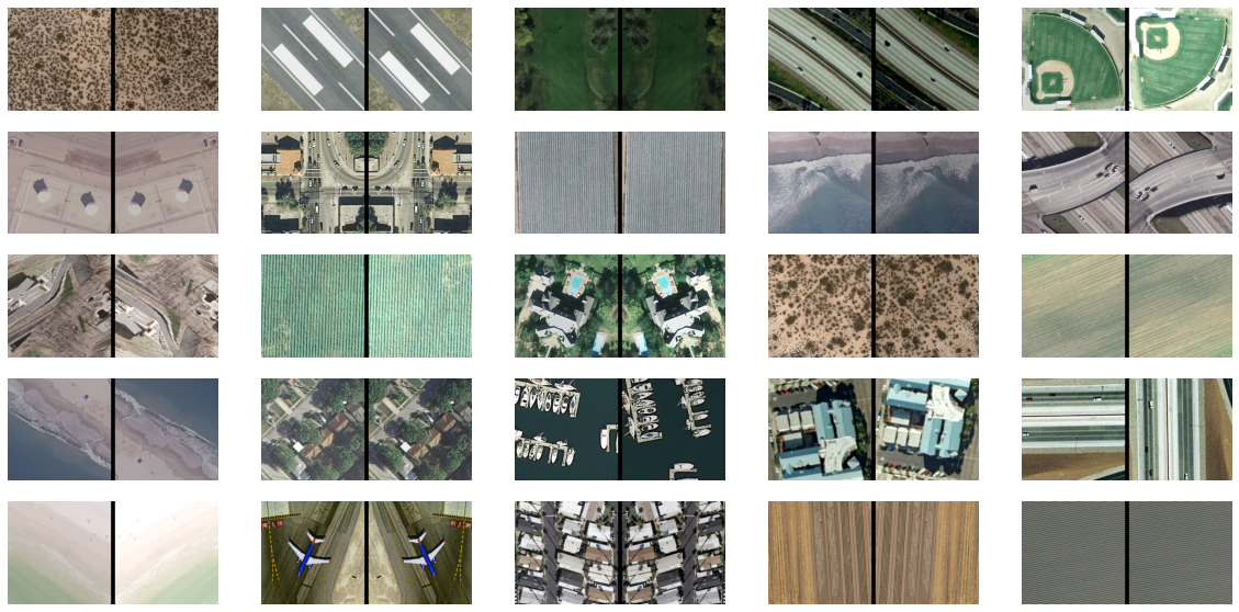
An important principle: augmentation is applied only to training data, never to validation or test data. Evaluation must always be performed on clean, unaugmented images to measure true generalization.

Results

Method	Train Loss	Val Loss	Test Loss	Train Acc	Val Acc	Test Acc
Without Augmentation	0.122	1.979	1.944	96.79%	54.81%	51.92%
With Augmentation	1.011	1.830	1.768	72.44%	58.41%	63.22%

Data augmentation delivers a +11.3 percentage point improvement on test accuracy (51.92% → 63.22%). Crucially, observe the shift in the train-test gap:

• Without augmentation: 96.79% train vs 51.92% test = 44.87 point gap
• With augmentation: 72.44% train vs 63.22% test = 9.22 point gap

The augmented model has lower training accuracy (the augmented samples are harder to memorize), but significantly better generalization. The train-test gap shrinks from 45 points to just 9 — a clear sign that the model is learning transferable patterns rather than memorizing specific training images.

6. Key Takeaways

1. Adam is the safest optimizer default, achieving the highest accuracy despite aggressive overfitting. For better loss calibration, SGD with momentum or learning rate scheduling can be a strong alternative.
2. Never initialize with zeros or constants. The symmetry-breaking property of random initialization (Glorot, He) is not optional — it is essential for gradient-based learning.
3. Glorot Uniform is a reliable default for most architectures. He Uniform shines specifically with deep ReLU networks without batch normalization.
4. Data augmentation is the single most impactful technique for small datasets. It improved test accuracy by +11.3 points while reducing the generalization gap by 35 points.
5. Choose domain-appropriate augmentations. For aerial/satellite images, rotations and flips are natural. For face recognition, they would be harmful. Always reason about what transformations preserve the semantic content.
6. TensorBoard is invaluable for comparing multiple experiments. Logging training runs makes it easy to compare curves, identify anomalies, and share results.