From Feature Functions to Neural Networks

Neural networks are often presented as a fundamentally new paradigm. In reality, they are a natural extension of the feature function approach we have been building throughout this series. A neural network is simply a composition of parameterized feature functions — each layer transforms its input, and the composition of many simple transformations produces a highly expressive model.

In this post, we first apply combined feature functions to the Mauna Loa CO2 dataset, then build an object-oriented framework for composable feature functions, and finally assemble them into single- and two-hidden-layer neural networks.

1. CO2 Prediction with Combined Features

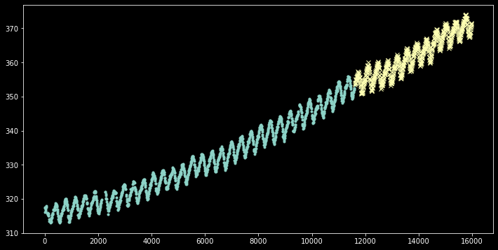
The Mauna Loa CO2 dataset presents a dual challenge: a long-term rising trend and annual seasonal oscillations. We combine different feature types to capture both patterns:

def get_feature_matrix(x):
    xf_a = get_feature_matrix_sin(x / 365.24, 1, 0)      # seasonal sine
    xf_b = get_feature_matrix_sin(x / 365.24, 1, 0.25)    # seasonal cosine
    xf_c = get_feature_matrix_poly(x / 16000, 1)           # linear trend
    xf_d = get_feature_matrix_relu(x / 16000, 10, 0)       # nonlinear trend
    return np.concatenate((xf_a, xf_b, xf_c, xf_d), axis=1)

This produces a 13-column feature matrix: 2 sinusoidal features (capturing the annual cycle), 1 polynomial feature (linear trend), and 10 ReLU features (allowing piecewise-linear trend adjustments).

Fitting a linear model on these features produces excellent results on the training set:

lrp = LinRegPredictor(M=13, l2=0.)
lrp.fit(xf_train, t_train)

print("Train loss:", lrp.score(xf_train, t_train))   # 0.50
print("Test loss:",  lrp.score(xf_test, t_test))      # 25.60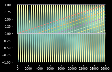

The model captures both the seasonal oscillation and the rising trend in the training data (train MSE = 0.50). However, the test loss is 50× worse (25.60). The ReLU features, being piecewise-linear, cannot extrapolate beyond the training range — the last three ReLU features have zero weights because they only activate in the test region. This highlights a fundamental limitation: hand-crafted features require domain knowledge about the extrapolation behavior.

2. The Forrester Function Benchmark

To study approximation quality more carefully, we switch to a standard synthetic test function — the Forrester function:

def forrester_function(x):
    return (6*x - 2)**2 * np.sin(12*x - 4)

x = np.linspace(0, 1, 101)
t = forrester_function(x)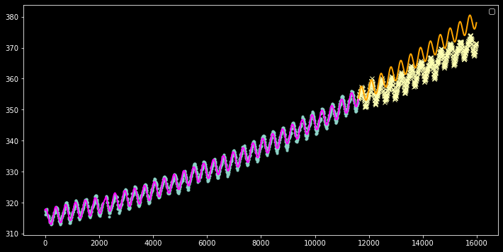

This function has a rich, non-trivial shape with a deep valley near x = 0.15 and a tall peak near x = 0.75. It serves as an excellent benchmark for comparing approximation methods.

3. Object-Oriented Feature Functions

Rather than defining feature matrices as standalone functions, we create an abstract base class that all feature functions inherit from. This enables composition — the output of one feature function becomes the input to the next:

class FeatureFunction:

    def __init__(self, theta=None):
        self._theta = None
        self.n_theta = 0

    def __call__(self, x):
        return self._calculate(x)

    def set_theta(self, theta):
        if theta is not None:
            self._theta = theta
            self.n_theta = np.size(theta)
        return self

    def _calculate(self, x):
        raise NotImplementedError

Every feature function has parameters (theta) that can be set externally, a __call__ method for easy invocation, and an abstract _calculate method that subclasses must implement.

FLinear: Matrix Multiplication Layer

class FLinear(FeatureFunction):

    def __init__(self, dim_in, dim_out, theta=None):
        self._dim_in = dim_in
        self._dim_out = dim_out
        self.set_theta(theta)

    def set_theta(self, theta):
        super().set_theta(theta)
        self._w = np.reshape(theta, (self._dim_in, self._dim_out))
        return self

    def _calculate(self, x):
        if np.ndim(x) == 1:
            x = x[:, np.newaxis]
        return x @ self._w

FReLU: Activation Function

class FReLU(FeatureFunction):

    def __init__(self):
        pass

    def _calculate(self, x):
        if np.ndim(x) == 1:
            x = x[:, np.newaxis]
        return np.fmax(0, x)

FBias: Additive Bias

class FBias(FeatureFunction):

    def __init__(self, theta):
        self.set_theta(theta)

    def set_theta(self, theta):
        super().set_theta(theta)
        self._b = np.reshape(theta, (1, -1))

    def _calculate(self, x):
        if np.ndim(x) == 1:
            x = x[:, np.newaxis]
        return x + self._b

These three building blocks are all we need. They compose naturally:

# Composing: input -> bias -> linear -> relu
result = relu(lin(bias(x0)))

4. Single Hidden Layer Network

By chaining our feature function classes, we can build a single-hidden-layer neural network:

input → bias₁ → ReLU → linear → bias₂ → output

class Predictor:

    def __init__(self, theta_bias1, theta_lin, theta_bias2, no_features):
        self.bias1 = FBias(theta=theta_bias1)
        self.relu = FReLU()
        self.lin = FLinear(no_features, 1, theta=theta_lin)
        self.bias2 = FBias(theta=theta_bias2)
        self._theta = np.concatenate((theta_bias1, theta_lin, theta_bias2))

    def fit(self, X, t, tol=0.001, opt_options=None):
        opt = scipy.optimize.minimize(self._loss, self._theta,
                                       (X, t), tol=tol, options=opt_options)
        self.set_theta(opt.x)

    def _loss(self, theta, X, t):
        n_samples = X.shape[0]
        y = self._predict(theta, X)
        return 0.5 * np.sum((y - t[:, np.newaxis]) ** 2) / n_samples

    def predict(self, X):
        z1 = self.bias1(X)
        z2 = self.relu(z1)
        z3 = self.lin(z2)
        return self.bias2(z3)

With 10 ReLU units, the single-layer network approximates the Forrester function:

p = Predictor(theta_bias1, theta_lin, theta_bias2, no_features=10)
p.fit(x, t, opt_options={"maxiter": 1000})
# Final loss: 0.2299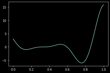

The fit captures the broad shape but with visible approximation errors. Because ReLU activations produce piecewise-linear outputs, a single layer can only create piecewise-linear functions — smooth curves require many segments or a different approach.

5. Two Hidden Layer Network

Adding a second hidden layer dramatically increases the network's expressiveness. The architecture becomes:

input → bias₁ → ReLU₁ → linear₁ → bias₂ → ReLU₂ → linear₂ → bias₃ → output

class Predictor2:

    def __init__(self, theta_bias1, theta_lin1, theta_bias2,
                 theta_lin2, theta_bias3, no_features1, no_features2):
        self.bias1 = FBias(theta_bias1)
        self.relu1 = FReLU()
        self.lin1 = FLinear(no_features1, no_features2, theta_lin1)
        self.bias2 = FBias(theta_bias2)
        self.relu2 = FReLU()
        self.lin2 = FLinear(no_features2, 1, theta_lin2)
        self.bias3 = FBias(theta_bias3)
        # ... fit and predict follow the same pattern

p2 = Predictor2(..., no_features1=10, no_features2=10)
p2.fit(x, t, opt_options={"maxiter": 1000})
# Final loss: 0.0408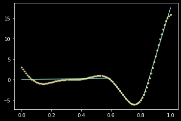

The two-layer network achieves a loss of 0.041 — nearly 6× better than the single-layer network's 0.230. Composing two piecewise-linear transformations creates piecewise-linear-of-piecewise-linear functions, which can approximate smooth curves much more closely.

Architecture	Hidden Units	Final Loss
Single hidden layer	10	0.2299
Two hidden layers	10 + 10	0.0408

6. Key Takeaways

"A neural network is just a composition of simple, parameterized transformations."

1. Feature functions are layers: FLinear is a dense layer. FReLU is an activation. FBias adds bias. Chaining them builds a neural network.
2. Depth increases expressiveness: A single-layer ReLU network produces piecewise-linear functions. Two layers compose these into much richer function families, achieving 6× lower loss on the Forrester benchmark.
3. Hand-crafted features have limits: The CO2 experiment shows that ReLU features cannot extrapolate. Neural networks learn features end-to-end but face similar challenges with out-of-distribution data.
4. The OOP design pattern — abstract base class with composable subclasses — mirrors how modern deep learning frameworks (PyTorch's nn.Module, TensorFlow's Keras layers) are actually structured.
5. Optimization is the bottleneck: Both networks use scipy.optimize.minimize with fixed iteration limits. Modern deep learning replaces this with stochastic gradient descent, which scales to millions of parameters.