Kaggle House Prices: A Complete Exploratory Data Analysis

The Kaggle House Prices competition is a rite of passage for aspiring data scientists. With 79 features describing almost every aspect of residential homes in Ames, Iowa, it demands thorough exploratory data analysis before any modeling can begin. In this post, we walk through a complete EDA pipeline: handling missing data, understanding distributions, encoding categorical variables, measuring feature importance, and engineering new features for regression.

1. Dataset Overview

The dataset contains 1,460 training instances with 81 attributes: 36 quantitative, 43 categorical, plus Id and SalePrice (the target).

train = pd.read_csv('../input/train.csv')

quantitative = [f for f in train.columns if train.dtypes[f] != 'object']
quantitative.remove('SalePrice')
quantitative.remove('Id')

qualitative = [f for f in train.columns if train.dtypes[f] == 'object']

print(f"Quantitative: {len(quantitative)}")    # 36
print(f"Qualitative:  {len(qualitative)}")     # 43

The quantitative features include lot dimensions, square footages, room counts, year built, and garage statistics. The qualitative features describe zoning, neighborhood, building type, quality ratings, and condition assessments.

2. Missing Data Analysis

Nineteen attributes have missing values, with five having over 50% missing:

missing = train.isnull().sum()
missing = missing[missing > 0]
missing.sort_values(inplace=True)
missing.plot.bar()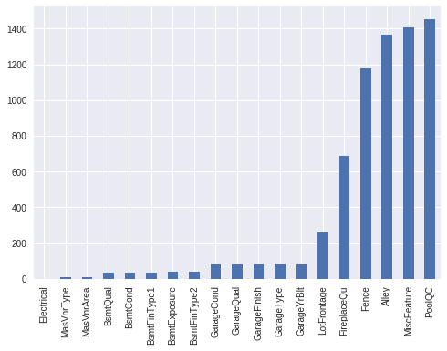

Most of the time, NA does not indicate data collection failure — it means the absence of the feature. A missing PoolQC means no pool; a missing Fence means no fence; a missing GarageType means no garage. Understanding this distinction is crucial for proper imputation.

3. Target Distribution

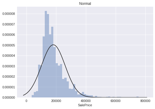
SalePrice does not follow a normal distribution. We fit three candidate distributions to assess the best transformation:

import scipy.stats as st

y = train['SalePrice']
sns.distplot(y, kde=False, fit=st.johnsonsu)    # Best fit
sns.distplot(y, kde=False, fit=st.norm)          # Poor fit
sns.distplot(y, kde=False, fit=st.lognorm)       # Decent fit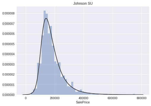

The Johnson SU distribution provides the best fit, capturing the right-skewed, peaked shape of home prices. The normal distribution fails badly — it is too symmetric. Before performing regression, the target must be transformed. While log transformation works well in practice, the Johnson SU transform achieves the closest match to normality.

Normality Testing

The Shapiro-Wilk test confirms that none of the 36 quantitative variables follow a normal distribution at the 0.01 significance level:

test_normality = lambda x: stats.shapiro(x.fillna(0))[1] < 0.01
normal = pd.DataFrame(train[quantitative]).apply(test_normality)
print(not normal.any())    # False -- all reject normality

4. Categorical Variable Analysis

For each of the 43 categorical variables, we create box plots showing the distribution of SalePrice across category values:

Key observations:

• Neighborhood has the largest impact — some neighborhoods (NridgHt, NoRidge, StoneBr) command significantly higher prices.
• Quality ratings (ExterQual, KitchenQual, BsmtQual) show clear ordinal relationships with price.
• SaleCondition = "Partial" (new homes) has the highest median price.
• Having a pool substantially increases property value.

ANOVA Feature Selection

We use ANOVA F-tests to quantify each categorical variable's influence on SalePrice. For each variable, we partition prices by category and test whether the group means are significantly different:

def anova(frame):
    anv = pd.DataFrame()
    anv['feature'] = qualitative
    pvals = []
    for c in qualitative:
        samples = [frame[frame[c] == cls]['SalePrice'].values
                   for cls in frame[c].unique()]
        pval = stats.f_oneway(*samples)[1]
        pvals.append(pval)
    anv['pval'] = pvals
    return anv.sort_values('pval')

a = anova(train)
a['disparity'] = np.log(1. / a['pval'].values)
sns.barplot(data=a, x='feature', y='disparity')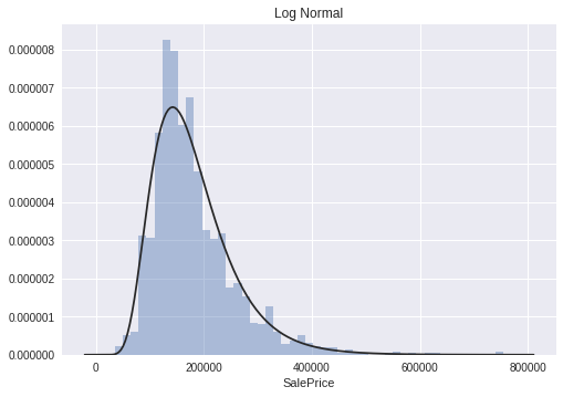

The top-ranked features — Neighborhood, ExterQual, KitchenQual, BsmtQual, GarageFinish — have extremely small p-values, indicating strong statistical evidence that their category values produce different price distributions.

5. Categorical Encoding

To include categorical variables in regression, we encode them numerically. Rather than one-hot encoding (which creates many sparse columns), we use mean-based ordinal encoding: categories are ranked by their mean SalePrice:

def encode(frame, feature):
    ordering = pd.DataFrame()
    ordering['val'] = frame[feature].unique()
    ordering.index = ordering.val
    ordering['spmean'] = frame[[feature, 'SalePrice']].groupby(feature).mean()['SalePrice']
    ordering = ordering.sort_values('spmean')
    ordering['ordering'] = range(1, ordering.shape[0] + 1)
    ordering = ordering['ordering'].to_dict()

    for cat, o in ordering.items():
        frame.loc[frame[feature] == cat, feature + '_E'] = o

This preserves the ordinal relationship between categories while producing a single numeric column per feature. For example, Neighborhood_E ranks neighborhoods from 1 (cheapest) to N (most expensive).

6. Correlation Analysis

We use Spearman rank correlation (rather than Pearson) because it captures monotonic relationships even when they are nonlinear:

features = quantitative + qual_encoded
spr = pd.DataFrame()
spr['feature'] = features
spr['spearman'] = [train[f].corr(train['SalePrice'], 'spearman') for f in features]

The strongest predictors of SalePrice:

Feature	Spearman r
OverallQual	~0.81
GrLivArea	~0.73
ExterQual_E	~0.72
GarageCars	~0.68
KitchenQual_E	~0.67

OverallQual is the single strongest predictor. Neighborhood has a large influence, partially due to intrinsic value and partially due to confounding — houses in the same neighborhood tend to share similar characteristics.

7. Feature Engineering

Based on the EDA findings, we engineer three types of new features:

Log Transforms

Applied to right-skewed features to reduce the influence of extreme values:

log_transform('GrLivArea')
log_transform('1stFlrSF')
log_transform('TotalBsmtSF')
log_transform('LotArea')
log_transform('LotFrontage')
log_transform('GarageArea')

Quadratic Terms

For features with nonlinear relationships to SalePrice:

quadratic('OverallQual')      # Clear nonlinear trend
quadratic('YearBuilt')         # Newer houses disproportionately expensive
quadratic('Neighborhood_E')    # Nonlinear neighborhood effect
quadratic('GrLivArea')         # Diminishing returns at extreme sizes

Boolean Indicators

Binary flags for presence/absence of features:

train['HasBasement'] = (train['TotalBsmtSF'] > 0).astype(int)
train['HasGarage']   = (train['GarageArea'] > 0).astype(int)
train['Has2ndFloor'] = (train['2ndFlrSF'] > 0).astype(int)
train['HasPool']     = (train['PoolArea'] > 0).astype(int)
train['IsNew']       = (train['YearBuilt'] > 2000).astype(int)

8. Regression Results

With all engineered features, we fit a LassoLarsCV model on log-transformed SalePrice:

features = quantitative + qual_encoded + boolean + qdr
lasso = linear_model.LassoLarsCV(max_iter=10000)
X = train[features].fillna(0.).values
Y = train['SalePrice'].values
lasso.fit(X, np.log(Y))

Ypred = np.exp(lasso.predict(X))
print("RMSLE:", error(Y, Ypred))    # 0.1097

An alternative approach using Ridge regression with Patsy formulas enables elegant specification of B-spline basis expansions and interaction terms:

Y, X = patsy.dmatrices(
    "SalePrice ~ GarageCars + np.log1p(BsmtFinSF1) + "
    "OverallQual + np.square(OverallQual) + "
    "Neighborhood_E:OverallQual + "
    "bs(OverallCond, df=7, degree=1) + ...",
    train.to_dict('list'))

ridge = linear_model.RidgeCV(cv=10)
ridge.fit(X, np.log(Y))
# RMSLE: 0.1160

The Lasso model achieves RMSLE ~0.110, while Ridge with splines and interactions achieves ~0.116. Adding quadratic terms improves the local score but can behave unstably on the leaderboard, suggesting potential overfitting to the training distribution.

9. Key Takeaways

1. EDA before modeling: Spending time understanding the data structure, distributions, and relationships pays dividends in feature engineering and model selection.
2. NA often means absence: In real estate data, missing values frequently indicate the lack of a feature (no pool, no garage), not a data collection error.
3. Transform the target: SalePrice is right-skewed. Log transformation makes it approximately normal, improving linear model performance.
4. Use Spearman over Pearson: Spearman rank correlation captures nonlinear monotonic relationships that Pearson misses.
5. Feature engineering is model-dependent: Quadratic terms help locally but may not generalize. Boolean indicators are more robust. The right features depend on the model family and the amount of training data.