Linear Regression and Curve Fitting from Scratch

Linear regression is the "Hello World" of machine learning — simple enough to understand completely, yet powerful enough to solve real problems. In this post, we first use scikit-learn's built-in LinearRegression to fit a line to data, then build the same model entirely from scratch to understand what happens under the hood.

We work with the sklearn diabetes dataset, isolating a single feature (BMI) to visualize the relationship between body mass index and disease progression.

1. Preparing the Data

We load the diabetes dataset and extract BMI as our sole input feature. Since many ML algorithms expect a 2D feature matrix of shape (n_samples, n_features), we reshape the 1D BMI array into a column vector:

from sklearn import datasets

diabetes_dataset = datasets.load_diabetes(as_frame=True)

# Extract BMI as a single feature column
x_bmi = diabetes_dataset["frame"]["bmi"].to_numpy()
x_bmi = x_bmi[:, np.newaxis]   # (442,) => (442, 1)

# Target: disease progression
t = diabetes_dataset["target"].to_numpy()   # (442,)

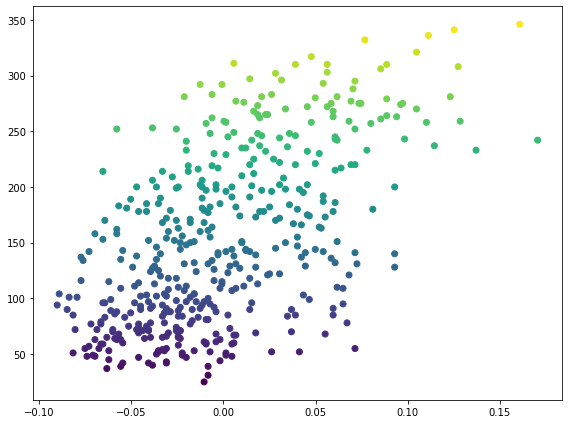
A scatter plot of BMI vs. disease progression reveals a noisy but positive trend — higher BMI values tend to correlate with more severe disease progression:

2. Linear Regression with Scikit-Learn

Scikit-learn makes fitting a linear model effortless. The LinearRegression class implements ordinary least squares (OLS), which finds the line that minimizes the sum of squared residuals:

from sklearn import linear_model

linreg = linear_model.LinearRegression()
linreg.fit(x_bmi, t)

# Generate predictions for plotting
x_lin = np.linspace(-0.5, 0.8, 200)[:, np.newaxis]
y_lin = linreg.predict(x_lin)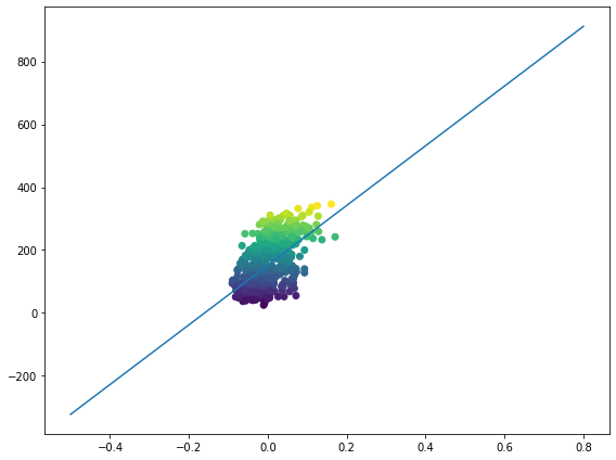

The fitted line passes through the center of the point cloud with a positive slope. The model parameters — slope (linreg.coef_) and intercept (linreg.intercept_) — are computed automatically during .fit().

3. Evaluation Metrics

Three standard metrics for regression models:

• Mean Squared Error (MSE): Average of squared differences between predictions and true values. Penalizes large errors quadratically.
• Mean Absolute Error (MAE): Average of absolute differences. More robust to outliers than MSE.
• R² Score: Proportion of variance in the target explained by the model. Ranges from 0 (no explanatory power) to 1 (perfect prediction).

from sklearn.metrics import mean_squared_error, mean_absolute_error, r2_score

y_pred = linreg.predict(x_bmi)

print("MSE:", mean_squared_error(t, y_pred))    # 3890.46
print("MAE:", mean_absolute_error(t, y_pred))    # 51.80
print("R2:",  r2_score(t, y_pred))               # 0.344

An R² of 0.344 means BMI alone explains about 34% of the variance in disease progression — meaningful, but far from the full picture. Additional features (age, blood pressure, serum measurements) would improve this substantially.

Manual Metric Implementation

Understanding what these metrics compute is important. Here they are implemented with pure NumPy:

def calculate_mse(y_true, y_pred):
    return np.mean((y_true - y_pred) ** 2)

def calculate_mae(y_true, y_pred):
    return np.mean(np.abs(y_true - y_pred))

def calculate_r2(y_true, y_pred):
    ss_res = np.sum((y_true - y_pred) ** 2)
    ss_tot = np.sum((y_true - y_true.mean()) ** 2)
    return 1 - ss_res / ss_tot

4. Building a Model from Scratch

Using sklearn is convenient, but to truly understand regression we need to build it ourselves. Every supervised ML model follows a four-step framework:

1. Feature extraction: Transform raw inputs into a feature matrix
2. Prediction function: Define y(w, x) = w₁ · x + w₀
3. Loss function: Quantify how far predictions are from truth (MSE)
4. Optimization: Find parameters w that minimize the loss

Step 1: Feature Extraction (Vandermonde Matrix)

For a linear model y = w₁x + w₀, we need both the feature values and a column of ones (for the intercept). NumPy's vander function creates exactly this — a Vandermonde matrix where column j contains x^M-1-j:

def get_features(data):
    x = data[:, 0]
    x_f = np.vander(x, 2)   # columns: [x^1, x^0] = [x, 1]
    return x_f

x_f = get_features(x_bmi)   # shape: (442, 2)

Step 2: Prediction Function

def predict(w, x):
    return x @ w              # matrix multiplication: (N, 2) @ (2,) => (N,)

w_init = np.array([1., 0.])  # initial guess

Step 3: Loss Function (MSE)

def L(w, x, t):
    n_samples = x.shape[0]
    y = predict(w, x)
    return np.sum((y - t) ** 2) / n_samples

Step 4: Optimization

We use scipy.optimize.minimize to find the weights that minimize the loss function. This is a general-purpose numerical optimizer that works with any differentiable loss:

from scipy.optimize import minimize

opt = minimize(L, w_init, args=(x_f, t))
w_opt = opt.x    # optimized weights

5. Comparing Initial vs. Optimized Weights

Plotting predictions from both the initial guess and the optimized weights illustrates the effect of training:

fig = plt.figure(figsize=(8, 6))
ax = fig.gca()

ax.scatter(x_bmi, t, c=t)
ax.plot(x_lin, predict(w_init, get_features(x_lin)), label="w_init")
ax.plot(x_lin, predict(w_opt, get_features(x_lin)), label="w_opt")
fig.legend()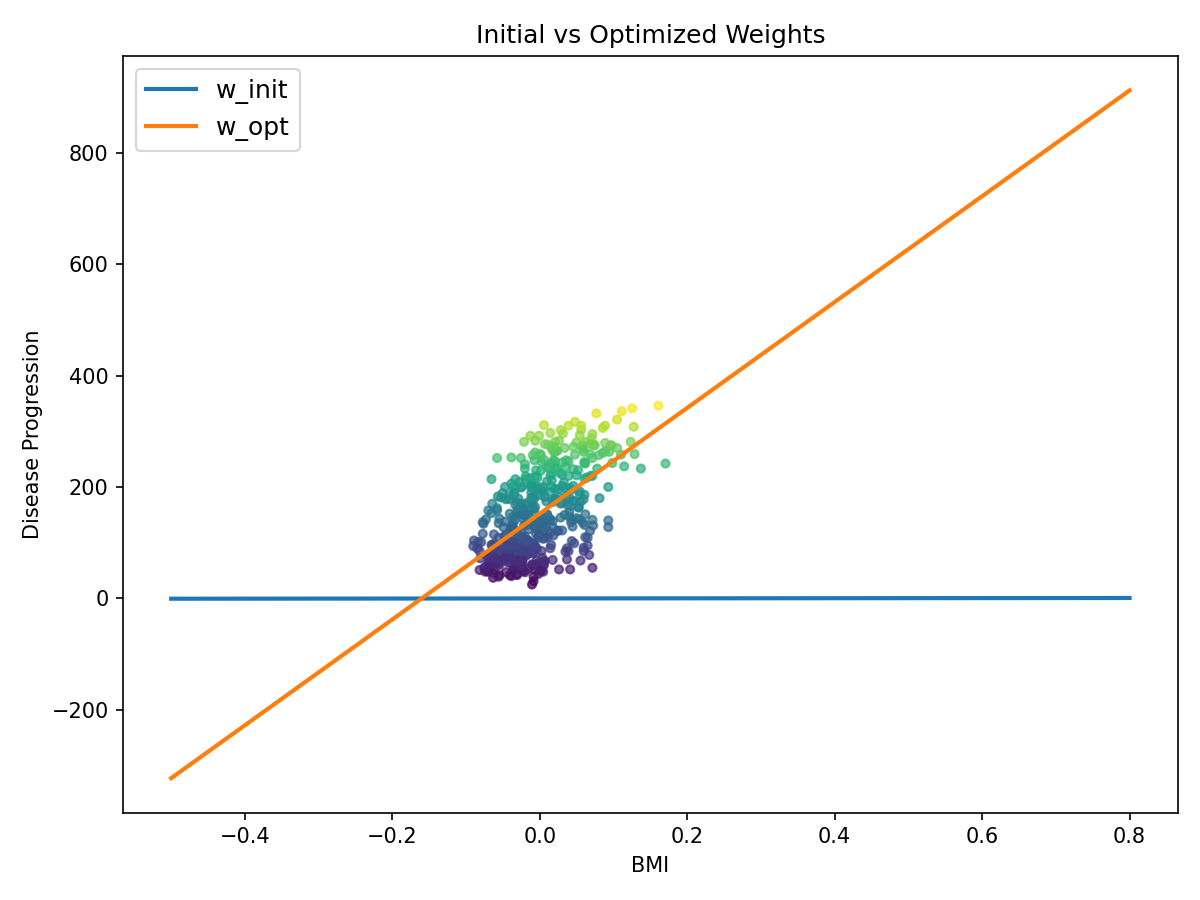

The initial weights produce an essentially flat line near zero (since BMI values are small standardized numbers). After optimization, the model converges to the same solution as sklearn's LinearRegression, confirming our from-scratch implementation is correct.

6. OOP Predictor Class

Finally, we encapsulate the entire pipeline into a reusable Python class that mimics sklearn's API pattern:

class LinRegPredictor:

    def __init__(self):
        self.w = np.array([1., 0.])

    def fit(self, X, t):
        opt = minimize(self._loss, self.w, args=(X, t))
        if opt.success:
            self.w = opt.x
        else:
            raise ValueError(f"Optimization failed: {opt.message}")

    def _loss(self, w, X, t):
        n_samples = X.shape[0]
        y = self._predict(w, X)
        return np.sum((y - t) ** 2) / n_samples

    def _predict(self, w, X):
        return X @ w

    def predict(self, X):
        return X @ self.w

lpr = LinRegPredictor()
lpr.fit(x_f, t)
print(lpr.w)    # matches linreg.coef_ and linreg.intercept_

This class design separates the public API (fit, predict) from internal methods (_loss, _predict). The underscore prefix is a Python convention for private methods. This pattern makes the class easy to extend — we can add regularization, different optimizers, or alternative loss functions by modifying just one or two methods.

7. Key Takeaways

1. The 4-step ML framework — features, predict, loss, optimize — applies to virtually every supervised learning algorithm, from linear regression to deep neural networks.
2. The Vandermonde matrix unifies linear and polynomial regression. For degree M, it produces columns [x^M-1, x^M-2, ..., x, 1], turning polynomial fitting into a linear algebra problem.
3. Sklearn is a black box — convenient but opaque. Building models from scratch develops the intuition needed to debug, extend, and choose the right approach for novel problems.
4. R² = 0.34 with one feature shows that a single predictor often captures only a fraction of the signal. Real-world problems typically require multiple features, feature engineering, or non-linear models.