Predicting Battery Life with LSTMs

Lithium-ion batteries degrade with every charge-discharge cycle. Knowing when a battery will reach the end of its useful life is critical for safety-critical applications like electric vehicles, aerospace systems, and grid-scale energy storage. In this project, we use Long Short-Term Memory (LSTM) networks to predict battery State of Health (SoH) from cycle-level measurements, using NASA's publicly available battery degradation dataset.

1. The NASA Battery Dataset

NASA's Prognostics Center of Excellence provides battery cycling data from controlled laboratory experiments. Each .mat file contains data for one battery, organized into three operation types:

• Charge cycles: Voltage, current, and temperature measured during constant-current/constant-voltage charging.
• Discharge cycles: Voltage, current, temperature, and capacity (Ah) measured during discharge until the cutoff voltage of 2.7V.
• Impedance measurements: Electrochemical impedance spectroscopy data at various frequencies.

We load data from four batteries (B0005, B0006, B0007, B0018) and extract the discharge cycle measurements:

from scipy.io import loadmat

def load_data(battery):
    mat = loadmat('../data/' + battery + '.mat')

    dataset = []
    capacity_data = []

    for i in range(len(mat[battery][0, 0]['cycle'][0])):
        row = mat[battery][0, 0]['cycle'][0, i]
        if row['type'][0] == 'discharge':
            data = row['data']
            capacity = data[0][0]['Capacity'][0][0]

            # Extract per-timestep measurements
            for j in range(len(data[0][0]['Voltage_measured'][0])):
                dataset.append([counter, ambient_temperature, date_time, capacity,
                    voltage, current, temperature, current_load, voltage_load, time_step])

            capacity_data.append([counter, ambient_temperature, date_time, capacity])

    return (pd.DataFrame(data=dataset, columns=[
                'cycle', 'ambient_temperature', 'datetime', 'capacity',
                'voltage_measured', 'current_measured', 'temperature_measured',
                'current_load', 'voltage_load', 'time']),
            pd.DataFrame(data=capacity_data, columns=[
                'cycle', 'ambient_temperature', 'datetime', 'capacity']))

dataset, capacity = load_data('B0005')

Each discharge cycle produces a time series of voltage, current, and temperature measurements, along with a single scalar capacity value that represents the total energy the battery delivered before reaching the cutoff voltage.

2. Capacity Degradation Analysis

Battery capacity decreases over charge-discharge cycles as the internal chemistry degrades. Plotting capacity versus cycle number reveals the characteristic capacity fade curve:

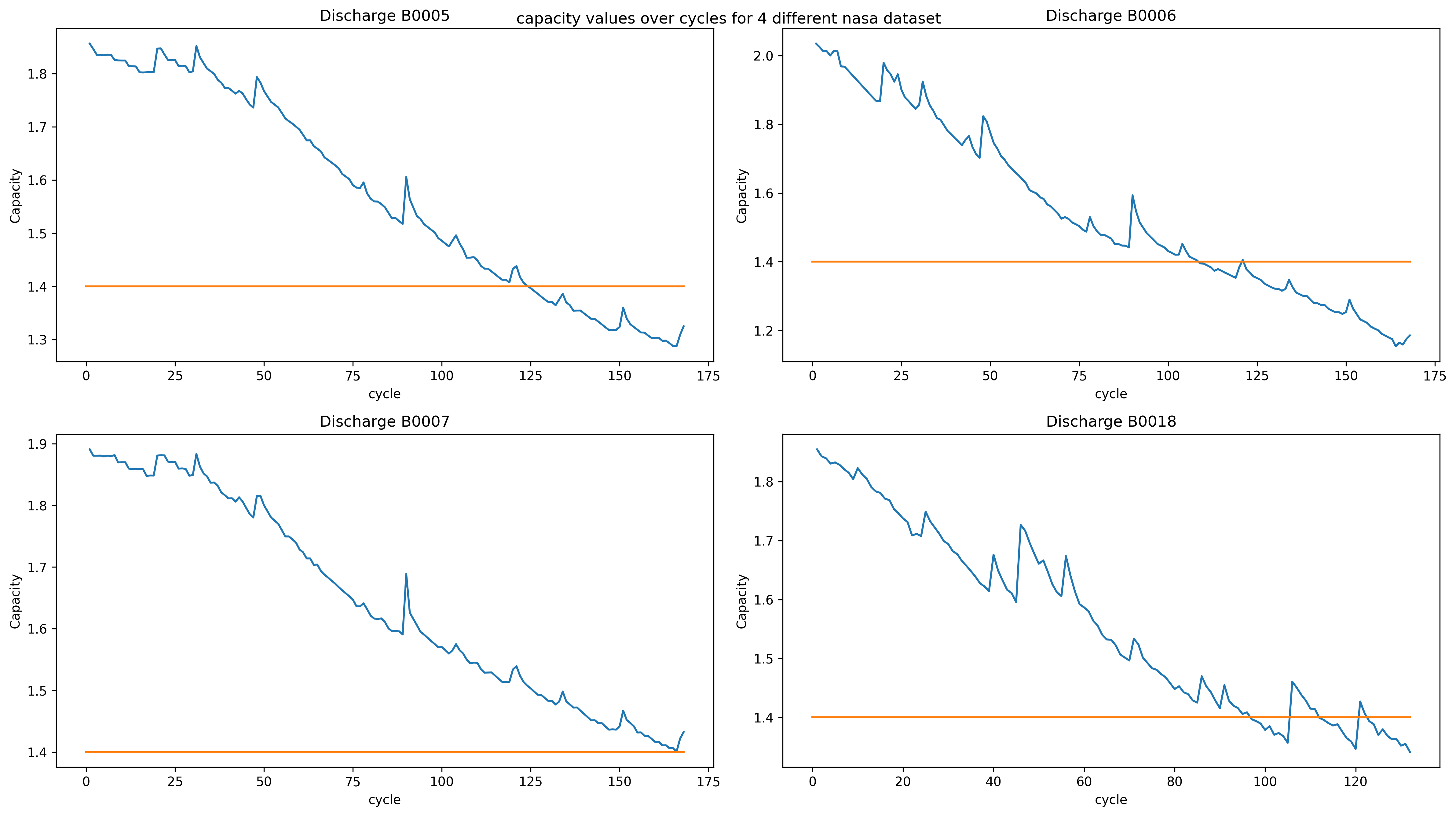
The horizontal line represents the end-of-life threshold at 70% of the initial capacity. When a battery crosses this line, it is considered degraded beyond useful service. Different batteries reach this threshold at different cycle numbers due to variations in manufacturing and operating conditions.

State of Health (SoH)

SoH is defined as the ratio of current capacity to initial capacity:

SoH = Capacity_current / Capacity_initial

max_C = dataset['capacity'][0]
dataset['SoH'] = dataset['capacity'] / max_C

SoH ranges from 1.0 (brand new) to 0.0 (completely degraded). In practice, batteries are replaced at SoH ≈ 0.7 (70%).

3. Feature Engineering

For the LSTM model, the input features are extracted from each discharge cycle's time series:

• Voltage measured: Terminal voltage during discharge
• Current measured: Current flowing through the battery
• Temperature measured: Battery surface temperature
• Current load: Current drawn by the external load
• Voltage load: Voltage measured at the load
• Time: Elapsed time during discharge

The target variable is the SoH, normalized to [0, 1]. All input features are also normalized to prevent scale-dependent bias in the neural network.

Data is organized into sliding windows of fixed length. Each window contains consecutive time steps from a discharge cycle, and the model learns to predict the SoH from the temporal patterns within the window.

4. LSTM Architecture

LSTMs are a variant of recurrent neural networks designed to capture long-range temporal dependencies. Unlike standard RNNs, LSTMs use gating mechanisms (forget gate, input gate, output gate) that control information flow, preventing the vanishing gradient problem.

Model 1: Stateful LSTM

model = Sequential()
model.add(CuDNNLSTM(64,
    kernel_initializer=init_glorot_uniform,
    recurrent_initializer=init_orthogonal,
    batch_input_shape=(10, window_size, number_of_features - 1),
    stateful=True,
    return_sequences=False))
model.add(Dense(64, 'tanh'))
model.add(Dense(1, 'tanh'))

Layer	Output Shape	Parameters
CuDNNLSTM (64 units)	(10, 64)	18,688
Dense (64, tanh)	(10, 64)	4,160
Dense (1, tanh)	(10, 1)	65

The stateful LSTM preserves its hidden state across batches. After each epoch, the state is manually reset. This allows the network to learn dependencies across multiple batches, which is important for long time series where a single batch cannot capture the full temporal context.

Model 2: Stateless LSTM

The same architecture with stateful=False. The hidden state resets at the start of each batch. This is simpler to train and may generalize better when the temporal dependencies are short-range.

Model 3: Stacked LSTM

model3 = Sequential()
model3.add(CuDNNLSTM(64,
    batch_input_shape=(10, window_size, number_of_features - 1),
    stateful=True,
    return_sequences=True))    # Pass full sequence to next LSTM
model3.add(CuDNNLSTM(64,
    stateful=True,
    return_sequences=False))   # Output only final hidden state
model3.add(Dense(64, 'tanh'))
model3.add(Dense(1, 'tanh'))

The stacked LSTM adds a second recurrent layer, allowing the network to learn hierarchical temporal features. The first LSTM outputs the full sequence (return_sequences=True), which becomes the input to the second LSTM. This increases the total parameter count to ~56,000 but provides more representational power for complex degradation patterns.

5. Training

The models are trained for 50 epochs with MSE loss and RMSE as the monitoring metric. Callbacks save the best model and log training history:

model.compile(optimizer='adam', loss='mse',
              metrics=[tf.keras.metrics.RootMeanSquaredError()])

history = model.fit(data_gen_train,
                    epochs=50,
                    callbacks=[model_checkpoint, epoch_saver])

Training converges rapidly — the loss drops from 0.376 in the first batch to 0.002 by the end of epoch 1, and continues improving to <0.0001 by epoch 3. The CuDNNLSTM layer (GPU-optimized) enables fast training even with the large number of time steps.

6. Evaluation and Prediction

The trained models are evaluated on train, validation, and test splits. Predictions are compared against actual SoH values:

predictions = model.predict(x, batch_size=1).flatten()

df = pd.DataFrame({
    'Predictions': predictions * 100,
    'Actuals': y * 100
})

mse = mean_squared_error(y, predictions)
r2 = r2_score(y, predictions)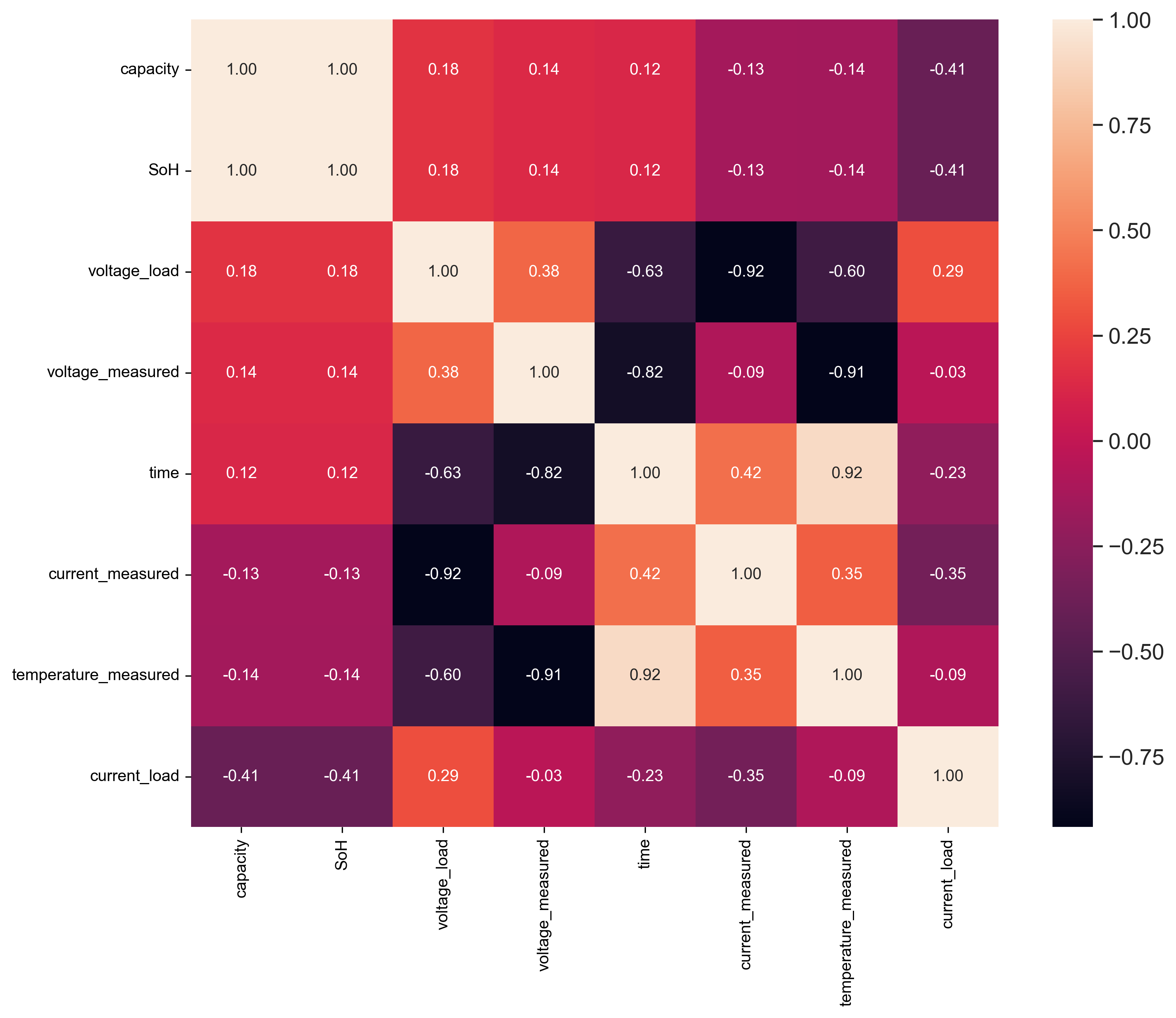

The LSTM tracks the actual SoH degradation closely, capturing both the overall downward trend and cycle-to-cycle variations. The R² score on the test set indicates excellent predictive accuracy.

7. Model Comparison

Model	Architecture	Parameters	Key Property
Model 1	LSTM(64) → Dense(64) → Dense(1)	22,913	Stateful
Model 2	LSTM(64) → Dense(64) → Dense(1)	22,913	Stateless
Model 3	LSTM(64) → LSTM(64) → Dense(64) → Dense(1)	56,193	Stacked + Stateful

The stateful model maintains hidden state across batches, allowing it to capture longer-range dependencies in the degradation trajectory. The stacked model provides additional depth for learning hierarchical temporal features, at the cost of more parameters and longer training time.

8. Key Takeaways

1. Battery degradation is a sequential problem: SoH depends on the entire history of charge-discharge cycles, not just the current measurement. LSTMs naturally capture this temporal dependency through their hidden state.
2. Feature engineering from raw signals: Extracting voltage, current, temperature, and capacity from NASA's .mat files requires careful parsing of the nested data structure. The quality of input features directly determines model performance.
3. Stateful vs. stateless: Stateful LSTMs can learn cross-batch dependencies but require careful batch management (manual state reset between epochs). Stateless LSTMs are simpler but may miss long-range patterns.
4. Stacking increases expressiveness: A two-layer LSTM learns hierarchical temporal features — the first layer extracts short-term patterns, the second combines them into longer-term trends.
5. Practical impact: Accurate SoH prediction enables predictive maintenance — replacing batteries before they fail, rather than after. This is crucial in aerospace (satellite batteries), automotive (EV range estimation), and grid storage applications.