The Complete Guide to Handling Missing Data

Missing data is one of the most common and insidious problems in real-world datasets. Simply deleting rows with NaN values may seem convenient, but it can introduce bias, reduce statistical power, and destroy valuable information. The right approach depends on why the data is missing and how much of it is gone.

In this post, we cover the complete missing data pipeline: detection, visualization, understanding missingness types, deletion strategies, simple imputation, group-aware imputation, and predictive methods including KNN and EM algorithm.

1. Guiding Principles

Before touching a single NaN value, keep three principles in mind:

1. Is the missingness random or not? The mechanism behind missing data determines which methods are valid.
2. NA does not always mean "lack": Sometimes missing values carry information (e.g., "no pool" in a housing dataset).
3. Beware information loss: Information can be deleted later if it does not affect the dataset, but it cannot be recovered once removed.

2. Detection Methods

Pandas provides several methods for systematically identifying missing values:

import numpy as np
import pandas as pd

V1 = np.array([1, 3, 6, np.NaN, 7, 1, np.NaN, 9, 0])
V2 = np.array([7, np.NaN, 5, 8, 12, np.NaN, np.NaN, 2, 3])
V3 = np.array([np.NaN, 12, 5, 6, 14, 7, np.NaN, 2, 31])
df = pd.DataFrame({"V1": V1, "V2": V2, "V3": V3})

# Count missing values per column
df.isnull().sum()
# V1: 2, V2: 3, V3: 2

# Total missing values in the dataset
df.isnull().sum().sum()    # 7

# Rows with at least one missing value
df[df.isnull().any(axis=1)]

# Rows with all values present (complete cases)
df[df.notnull().all(axis=1)]

3. Visualization with missingno

The missingno library provides three powerful visualizations for understanding the structure of missing data:

Bar Chart

import missingno as msno

msno.bar(df)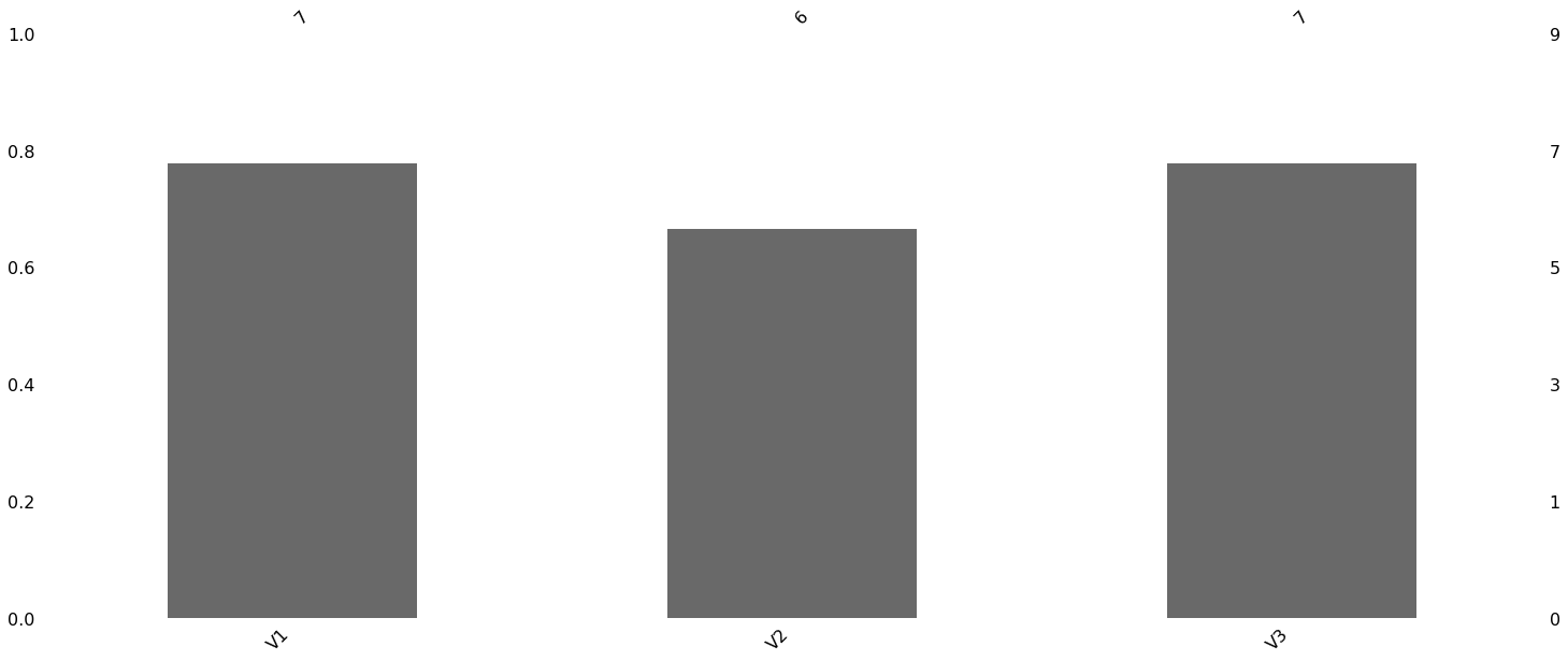

The bar chart gives an at-a-glance view of completeness per column. V2 has the most missing values (3 out of 9 rows).

Matrix Plot

msno.matrix(df)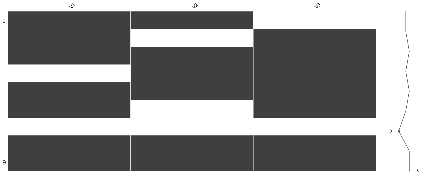

The matrix plot reveals patterns in missingness. Each row is a horizontal band; white gaps indicate missing values. Row 6 is entirely white (all three columns are NaN), suggesting a systematic data collection failure for that observation.

Correlation Heatmap

Applied to a larger dataset (Seaborn's planets dataset with 1,035 rows), the missingness correlation heatmap reveals dependencies between missing columns:

import seaborn as sns
df_planets = sns.load_dataset('planets')

msno.heatmap(df_planets)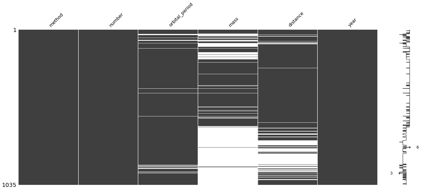

Key finding: mass and distance have a missingness correlation of 0.5, meaning when mass is missing, distance is also likely missing. This is strong evidence that the data is not Missing Completely At Random (MCAR) — the missingness has structure.

4. Types of Missing Data

• MCAR (Missing Completely At Random): Missingness is independent of both observed and unobserved data. Example: a lab instrument randomly malfunctions. Deletion is safe but wasteful.
• MAR (Missing At Random): Missingness depends on observed data but not on the missing values themselves. Example: younger patients are less likely to have cholesterol measured. Imputation using observed variables is appropriate.
• MNAR (Missing Not At Random): Missingness depends on the unobserved values. Example: patients with very high blood pressure are less likely to report it. The hardest case — requires domain knowledge or modeling assumptions.

5. Deletion Strategies

Pandas dropna() provides flexible deletion options:

# Drop rows where ANY value is NaN (listwise deletion)
df.dropna()

# Drop rows where ALL values are NaN
df.dropna(how="all")

# Drop COLUMNS where ANY value is NaN
df.dropna(axis=1)

# Drop COLUMNS where ALL values are NaN
df.dropna(axis=1, how="all")

# Permanent deletion (modifies df in place)
df.dropna(axis=1, how="all", inplace=True)

When to use deletion:

• The data is MCAR and the fraction of missing values is small (<5%)
• Entire rows or columns are empty and carry no information
• You have abundant data and can afford to lose some observations

6. Simple Imputation

Replace missing values with a summary statistic of the observed values:

# Fill with zero
df["V2"].fillna(0)

# Fill with column mean
df["V1"].fillna(df["V1"].mean())

# Fill with column median (more robust to outliers)
df["V3"].fillna(df["V3"].median())

# Fill ALL columns with their respective means
df.apply(lambda x: x.fillna(x.mean()), axis=0)

Group-Aware Imputation

The company-wide average salary may not be appropriate for every department. Group-aware imputation fills missing values using group-specific statistics:

df = pd.DataFrame({
    "salary": [1, 3, 6, np.NaN, 7, 1, np.NaN, 9, 15],
    "department": ["IT", "IT", "IK", "IK", "IK", "IK", "IK", "IT", "IT"]
})

# Mean salary by department
df.groupby("department")["salary"].mean()
# IK: 4.67,  IT: 7.00

# Fill NaN with department-specific mean
df["salary"].fillna(
    df.groupby("department")["salary"].transform("mean")
)

The IK department employee gets 4.67, while the IT employee gets 7.00 — much more accurate than a global mean of 5.86.

7. Categorical Variable Imputation

For categorical variables, mean/median imputation does not apply. Instead:

# Fill with mode (most frequent category)
df["department"].fillna(df["department"].mode()[0])

# Forward fill: propagate last valid observation forward
df["department"].fillna(method="ffill")

# Backward fill: use next valid observation
df["department"].fillna(method="bfill")

Forward and backward fill are particularly useful for time series data where the most recent known value is a reasonable estimate.

8. Predictive Imputation Methods

When the missingness is not random, simple statistics are not enough. Predictive methods use the relationships between variables to estimate missing values.

KNN Imputation

For each row with missing values, find the k most similar complete rows (nearest neighbors) and impute using their values:

from ycimpute.imputer import knnimput

# Load Titanic dataset (177 missing age values out of 891)
df = sns.load_dataset('titanic')
df = df.select_dtypes(include=['float64', 'int64'])

n_df = np.array(df)
dff = knnimput.KNN(k=4).complete(n_df)

# Verify: no missing values remain
pd.DataFrame(dff, columns=list(df)).isnull().sum()
# All zeros

KNN imputation works well when similar observations exist in the dataset and when the feature space is not too high-dimensional.

EM Algorithm

The Expectation-Maximization algorithm iteratively estimates the missing values (E-step) and model parameters (M-step), converging to a maximum likelihood solution:

from ycimpute.imputer import EM

dff = EM().complete(n_df)

# Verify: all missing values filled
pd.DataFrame(dff, columns=list(df)).isnull().sum()
# All zeros

EM assumes the data follows a parametric distribution (typically multivariate Gaussian). It is more principled than KNN but can be sensitive to the distributional assumption.

9. Decision Framework

Choosing the right approach depends on the missingness mechanism and the fraction of missing data:

Scenario	Recommended Approach
MCAR, <5% missing	Listwise deletion or mean imputation
MAR, moderate missing	Group-aware imputation or KNN
MAR, substantial missing	EM algorithm or multiple imputation
MNAR	Domain-specific modeling, sensitivity analysis
Entire column >50% missing	Consider dropping the column entirely
Categorical variable	Mode imputation, or add "MISSING" category
Time series	Forward fill or interpolation

10. Key Takeaways

1. Understand the mechanism first: Is the data MCAR, MAR, or MNAR? The missingno heatmap helps diagnose this by revealing correlations between missing patterns.
2. Visualize before acting: The missingno matrix and bar charts reveal patterns that summary statistics miss, such as rows where all values are missing simultaneously.
3. Simple methods have their place: Mean/median imputation is fast and often good enough when the fraction of missing data is small and MCAR holds.
4. Group-aware imputation is often better: Using group-specific statistics (e.g., department-level salary mean) preserves more of the data's structure than global statistics.
5. Predictive methods for complex missingness: KNN and EM use the full multivariate structure of the data, producing better estimates when variables are correlated and missingness is not random.