Multi-Layer Perceptron (MLP) for Image Classification

The Multi-Layer Perceptron is the foundational architecture of deep learning. Before convolutional networks, recurrent networks, or transformers, there was the MLP — a fully connected feedforward network that maps inputs to outputs through a series of nonlinear transformations. Understanding its strengths and limitations on image data provides the essential motivation for more specialized architectures.

In this post, we build an MLP for image classification on the Fashion MNIST dataset, examine its training dynamics, analyze where it succeeds and fails, and demonstrate a critical limitation: the lack of spatial invariance.

1. The Dataset: Fashion MNIST

Fashion MNIST is a dataset of Zalando's article images, designed as a drop-in replacement for the classic MNIST digits. It consists of 70,000 grayscale images (28×28 pixels) across 10 clothing categories:

Class	Description
0	T-shirt/top
1	Trouser
2	Pullover
3	Dress
4	Coat
5	Sandal
6	Shirt
7	Sneaker
8	Bag
9	Ankle boot

We split the original training set into training (54,000) and validation (6,000) subsets, keeping the 10,000 test images untouched:

(x_train, y_train), (x_test, y_test) = fashion_mnist.load_data()

# Hold out 10% as validation set
n_val = int(0.1 * len(x_train))
x_val, x_train = x_train[:n_val], x_train[n_val:]
y_val, y_train = y_train[:n_val], y_train[n_val:]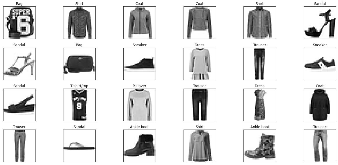

2. Data Preprocessing and Generators

We normalize pixel values to [0, 1] and expand dimensions for the channel axis:

x_train = np.expand_dims(x_train, axis=-1).astype("float32") / 255.0
x_val   = np.expand_dims(x_val, axis=-1).astype("float32") / 255.0
x_test  = np.expand_dims(x_test, axis=-1).astype("float32") / 255.0

Why Use Data Generators?

The naive approach of loading an entire dataset into memory works for small datasets like Fashion MNIST, but breaks down when dealing with real-world data (satellite imagery, medical scans, video frames). A data generator loads data in batches on-the-fly, providing:

• Memory efficiency: Only one batch resides in memory at a time
• Epoch-level shuffling: Data ordering changes each epoch, reducing memorization
• On-the-fly augmentation: Transformations can be applied dynamically without storing augmented copies

Keras provides two approaches: the built-in ImageDataGenerator class (convenient for standard augmentations), and custom generators by subclassing keras.utils.Sequence (flexible for any data format or transformation):

class DataGenerator(keras.utils.Sequence):
    def __init__(self, batch_size, data, labels, shuffle=True):
        self.batch_size = batch_size
        self.data = data
        self.labels = labels
        self.shuffle = shuffle

    def on_epoch_end(self):
        if self.shuffle:
            self.data, self.labels = shuffle(self.data, self.labels)

    def __len__(self):
        return self.data.shape[0] // self.batch_size

    def __getitem__(self, idx):
        i = idx * self.batch_size
        return self.data[i:i+self.batch_size], self.labels[i:i+self.batch_size]

data_gen_train = DataGenerator(batch_size=32, data=x_train, labels=y_train)
data_gen_val   = DataGenerator(batch_size=32, data=x_val, labels=y_val)

3. MLP Architecture

An MLP treats each image as a flat vector of pixels. For a 28×28 image, that means 784 input features, with no notion of spatial locality, adjacency, or structure. Our architecture:

• Input: Flatten layer — reshapes (28, 28, 1) to a 784-dimensional vector
• Hidden layer 1: 100 neurons, ReLU activation
• Hidden layer 2: 100 neurons, ReLU activation
• Hidden layer 3: 100 neurons, ReLU activation
• Output: 10 neurons, Softmax activation (one per class)

def get_model(hidden_layers, n_classes):
    model = Sequential()
    model.add(Flatten(input_shape=(28, 28, 1)))
    for i in hidden_layers:
        model.add(Dense(i, activation=tf.nn.relu))
    model.add(Dense(n_classes, activation=tf.nn.softmax))
    return model

model = get_model(hidden_layers=[100, 100, 100], n_classes=10)

The model summary reveals a total of 99,710 trainable parameters:

Layer (type)                 Output Shape       Param #
==========================================================
flatten (Flatten)            (None, 784)        0
dense (Dense)                (None, 100)        78,500
dense_1 (Dense)              (None, 100)        10,100
dense_2 (Dense)              (None, 100)        10,100
dense_3 (Dense)              (None, 10)         1,010
==========================================================
Total params: 99,710

Notice that 78,500 out of 99,710 parameters (79%) are concentrated in the first dense layer. This is a direct consequence of flattening: the 784-dimensional input vector connecting to 100 neurons requires 784 × 100 + 100 = 78,500 parameters. This front-heavy distribution is a hallmark of MLPs on image data and becomes untenable at higher resolutions.

4. Training and Analysis

We train with the Adam optimizer, sparse categorical cross-entropy loss, and two essential callbacks:

model.compile(optimizer='adam',
              loss=tf.keras.losses.SparseCategoricalCrossentropy(),
              metrics=['accuracy'])

callbacks = [
    ModelCheckpoint("classification_model.h5",
                    mode="max", save_best_only=True,
                    monitor="val_accuracy", verbose=1),
    EarlyStopping(patience=200, verbose=1, mode="auto")
]

Training Curves

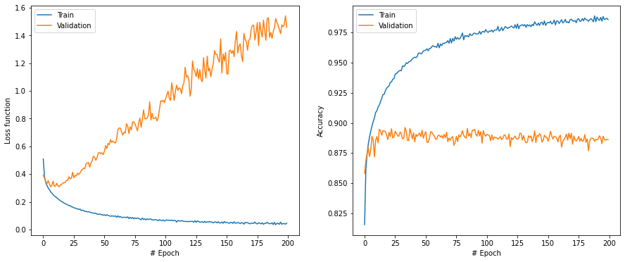
The training curves tell a dramatic story of severe overfitting:

• Training loss drops to near zero (~0.04), while validation loss explodes to over 1.4 by epoch 200.
• Training accuracy reaches ~97.5%, but validation accuracy plateaus around 89% and begins to fluctuate.
• The divergence begins as early as epoch 25, with the gap widening continuously thereafter.

This pattern is characteristic of a model that memorizes the training data rather than learning generalizable patterns. The MLP, with no inductive bias for spatial structure, relies on brute-force memorization of pixel positions.

Evaluation Results

Split	Loss	Accuracy
Train	0.1109	95.64%
Validation	0.4429	89.64%
Test	0.4685	89.23%

The ~6.4% gap between training and test accuracy, combined with a 4x difference in loss values, confirms the model is significantly overfitting. Best checkpoint weights (from the epoch with highest validation accuracy) partially mitigate this, but the underlying capacity problem remains.

5. Prediction Analysis

Visualizing predictions alongside confidence bars provides insight into the model's behavior. Green labels indicate correct predictions; red indicates misclassifications:

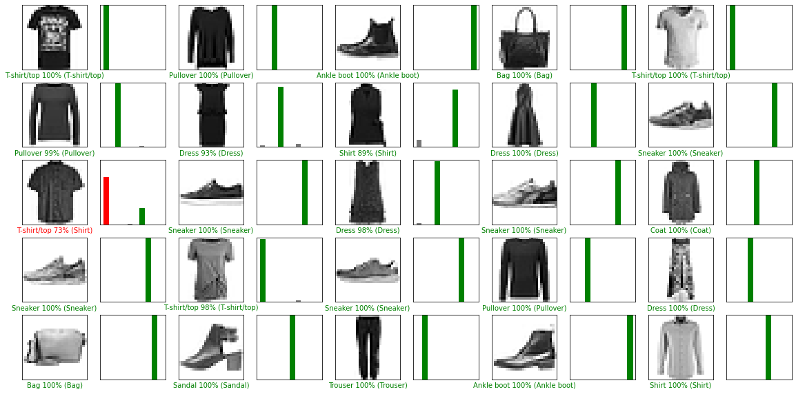
Several patterns emerge:

• The model is highly confident on easy classes like Trouser, Bag, and Sneaker (100% confidence).
• Confusion between similar classes is evident — the model predicts "T-shirt/top" at 73% confidence for an image that is actually a Shirt. These two classes are visually very similar and represent the hardest discrimination task in this dataset.
• Even correct predictions sometimes have lower confidence (e.g., Shirt at 89%), revealing the model's uncertainty on ambiguous items.

6. The Rotation Problem

Perhaps the most revealing experiment is testing the model's response to a simple geometric transformation. We take an image correctly classified as "Dress" and apply a 30-degree rotation:

from scipy.ndimage.interpolation import rotate

image_rot = rotate(image[0, ..., 0], angle=30, reshape=False)

# Original prediction: Dress (correct)
# Rotated prediction:  Bag   (incorrect!)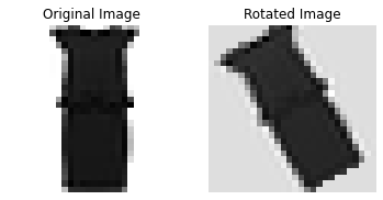

The original image is correctly classified as "Dress", but after a mere 30-degree rotation, the model predicts "Bag". This failure is not a bug — it is a fundamental architectural limitation.

An MLP has no notion of spatial structure. It treats each pixel as an independent feature at a fixed position. Moving or rotating the content shifts pixels to entirely different positions in the flattened vector, creating an input the network has never seen.

This is precisely the motivation for Convolutional Neural Networks (CNNs), which introduce:

• Local connectivity: Each neuron sees only a small spatial neighborhood, not the entire image.
• Weight sharing: The same filter is applied across all spatial positions, providing translation equivariance.
• Hierarchical feature extraction: Deeper layers compose local features into increasingly abstract representations.

7. Key Takeaways

1. MLPs can classify images, but poorly: 89% test accuracy on Fashion MNIST is respectable but leaves significant room for improvement. The severe overfitting (97.5% train vs 89% test) shows the model compensates for lack of structure with memorization.
2. The flatten bottleneck: Converting 2D images to 1D vectors destroys all spatial relationships. Neighboring pixels that form edges, textures, and shapes lose their geometric meaning.
3. No geometric invariance: MLPs are sensitive to translation, rotation, and scaling. A rotated dress becomes unrecognizable because pixels have shifted to different positions in the input vector.
4. Data generators are essential: Even for in-memory datasets, generators establish a pattern that scales to arbitrarily large data and enables on-the-fly augmentation.
5. Monitor the generalization gap: The divergence between training and validation loss is the most important diagnostic signal during training. When this gap widens, the model is memorizing rather than learning.

These limitations set the stage for our next topic: Convolutional Neural Networks, which address each of these shortcomings through architectures designed specifically for spatial data.