Polynomial Regression, Overfitting, and Regularization

A linear model can only capture straight-line relationships. When the true underlying function is curved — as it almost always is in practice — we need more flexible models. Polynomial regression extends linear regression by adding powers of the input as features, but this flexibility comes with a cost: overfitting.

In this post, we generate synthetic sine data with noise, sweep polynomial degrees to visualize overfitting, introduce Ridge (L2) and Lasso (L1) regularization, explore alternative feature functions, and apply everything to real-world Mauna Loa CO2 data.

1. Synthetic Data: Noisy Sine

We model the common scenario of observing a noisy signal and trying to recover the true function. The noise follows an additive Gaussian model:

t_i = y(x_i) + ε_i,   where   ε_i ~ N(0, σ²)

np.random.seed(1001)
sigma = 0.1

N_train = 16
x_train = np.random.rand(N_train)
t_train = np.sin(2. * x_train * np.pi) + np.random.randn(N_train) * sigma

N_test = 32
x_test = np.random.rand(N_test)
t_test = np.sin(2. * x_test * np.pi) + np.random.randn(N_test) * sigma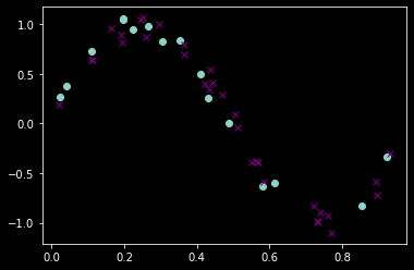

The green curve is the true function y = sin(2πx). The shaded region represents the 2σ confidence band — we expect most observations to fall within this range. Training points (circles) and test points (x-marks) follow the sine shape with small Gaussian perturbations.

2. The Analytic Solution

For linear models, we can bypass numerical optimization entirely. Setting the derivative of the MSE loss to zero yields the normal equation:

w_opt = (X^TX)^-1 X^Tt

The term (X^TX)^-1X^T is called the Moore-Penrose pseudoinverse, available as numpy.linalg.pinv:

class LinRegPredictor:

    def __init__(self, M):
        self.w = np.zeros(M)

    def fit(self, X, t):
        self.w = np.linalg.pinv(X) @ t

    def predict(self, X):
        return X @ self.w

    def score(self, X, t):
        y_pred = self.predict(X)
        return np.mean((t - y_pred) ** 2)

3. Polynomial Regression via Vandermonde Matrices

A Vandermonde matrix of degree M converts scalar inputs into polynomial features. For each input x, it produces the row [x^M-1, x^M-2, ..., x, 1]:

def get_feature_matrix_poly(x, M=2):
    return np.vander(x, M)

With M = 4, the model fits a cubic polynomial. The prediction closely follows the true sine shape:

M = 4
lrp = LinRegPredictor(M)
xf_train = get_feature_matrix_poly(x_train, M)
lrp.fit(xf_train, t_train)

print("Train loss:", lrp.score(xf_train, t_train))   # 0.0049
print("Test loss:",  lrp.score(xf_test, t_test))      # 0.0151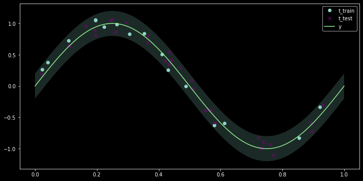

4. Overfitting: The Polynomial Degree Sweep

What happens when we increase M from 1 to 16 (the number of training points)? We systematically evaluate train and test loss for every degree:

scores = []
for M in range(1, N_train + 1):
    lrp = LinRegPredictor(M)
    xf_train = get_feature_matrix_poly(x_train, M)
    xf_test = get_feature_matrix_poly(x_test, M)
    lrp.fit(xf_train, t_train)
    scores.append([M, lrp.score(xf_train, t_train),
                      lrp.score(xf_test, t_test)])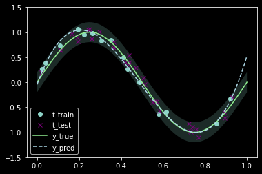

This is the classic overfitting U-curve:

• Training loss decreases monotonically — more parameters always allow a better fit to the training data.
• Test loss initially decreases (the model learns the true pattern), reaches a minimum around M ≈ 7, then explodes as the polynomial begins fitting noise rather than signal.
• At M = 16, the model has as many parameters as training points — it passes through every point exactly (zero training loss) but produces wild oscillations between them.

Degree M	Train Loss	Test Loss
M = 1	0.333	0.292
M = 4	0.005	0.015
M = 7	0.004	0.012
M = 16	≈ 0	4,556,000

5. Ridge Regression (L2 Regularization)

Regularization combats overfitting by penalizing large weight values. Ridge regression adds an L2 penalty to the loss:

L(w) = ½ ||Xw - t||² + ½λ ||w||²

The closed-form solution becomes:

w_opt = (X^TX + λI)^-1 X^Tt

The regularization parameter λ controls the trade-off between fitting the data and keeping weights small:

class LinRegPredictor:

    def __init__(self, M, l2=0.):
        self.w = np.zeros(M)
        self.l2 = l2

    def fit(self, X, t):
        n_features = X.shape[1]
        a = X.T @ X + self.l2 * np.eye(n_features)
        b = X.T @ t
        self.w, _, _, _ = np.linalg.lstsq(a, b, rcond=None)

M = 10
lrp = LinRegPredictor(M, l2=0.0001)
lrp.fit(xf_train, t_train)

print("Train loss:", lrp.score(xf_train, t_train))   # 0.0041
print("Test loss:",  lrp.score(xf_test, t_test))      # 0.0140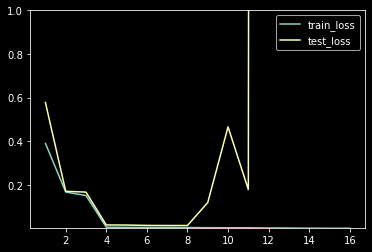

With λ = 0.0001, a degree-10 polynomial achieves better test loss (0.014) than the unregularized degree-7 model (0.015). The regularization keeps the weights bounded, preventing the wild oscillations we saw at high degrees.

6. Lasso Regression (L1 Regularization)

Lasso uses the L1 norm instead of L2. This promotes sparsity — some weights are driven exactly to zero, effectively performing feature selection:

L(w) = ½ ||Xw - t||² + λ₁ ||w||₁

Unlike Ridge, Lasso has no closed-form solution and requires iterative optimization. The resulting weights tend to have many zero entries, identifying which polynomial terms are most important for the fit.

7. Alternative Feature Functions

Polynomials are not the only way to create features. Three alternatives that are widely used in machine learning:

ReLU Features

Φ_relu(x - c) = max(0, x - c)

def get_feature_matrix_relu(x, M=1):
    c = np.linspace(0, 1, M)
    return np.fmax(x[:, np.newaxis] - c, 0)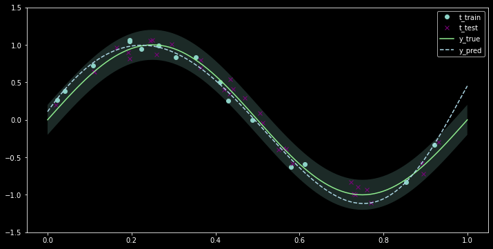

ReLU features are "hockey stick" functions that activate at different positions. A linear combination of many ReLUs creates piecewise-linear approximations.

Sinusoidal Features

Φ_sin(x) = sin(2πfx + 2πd)

def get_feature_matrix_sin(x, M, d=0.):
    f = 2. * np.pi * np.linspace(1, M + 1, M)
    return np.sin(np.outer(x, f) + 2 * np.pi * d)

Squared Exponential (Gaussian RBF) Features

Φ_SE(x - c) = exp(-(x - c)² / l²)

def get_feature_matrix_se(x, M, l=0.1):
    c = np.linspace(0, 1, M)
    dx = x[:, np.newaxis] - c
    return np.exp(-dx ** 2 / l ** 2)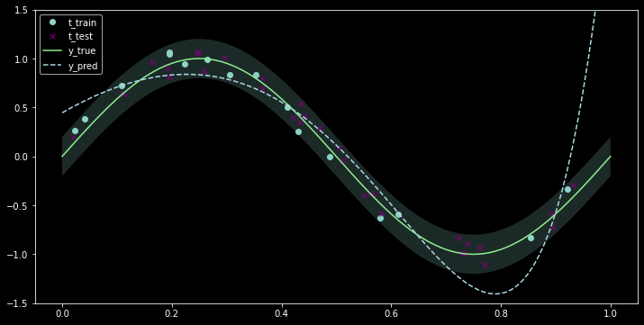

Combining Features

The real power comes from concatenating different feature types. Combining 5 ReLU, 3 sine (phase 0), 3 sine (phase π/2), and 10 SE features gives a 21-dimensional feature matrix:

def get_feature_matrix_concat(x):
    xf_a = get_feature_matrix_relu(x, 5)
    xf_b = get_feature_matrix_sin(x, 3)
    xf_c = get_feature_matrix_sin(x, 3, 0.25)
    xf_d = get_feature_matrix_se(x, 10, 0.2)
    return np.concatenate((xf_a, xf_b, xf_c, xf_d), axis=1)

# Fit with L1 + L2 regularization
lrp = LinRegPredictor(21, l2=0.001, l1=0.001)
lrp.fit(xf_train, t_train)

print("Train loss:", lrp.score(xf_train, t_train))   # 0.0028
print("Test loss:",  lrp.score(xf_test, t_test))      # 0.0159

8. Real-World Data: Mauna Loa CO2

We apply these techniques to a genuinely challenging dataset: weekly atmospheric CO2 concentrations measured at the Mauna Loa Observatory in Hawaii from 1958 to 2001 (the famous Keeling Curve).

from sklearn.datasets import fetch_openml
co2 = fetch_openml(data_id=41187, as_frame=True)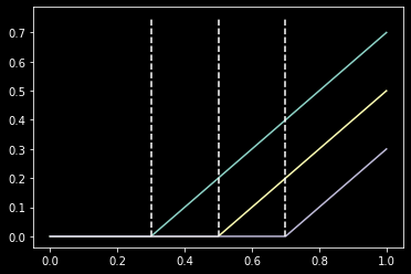

The data exhibits two distinct patterns: a long-term upward trend (from ~316 ppm in 1958 to ~371 ppm in 2001) and annual seasonal oscillations driven by the photosynthesis cycle. This makes it an excellent testbed for feature engineering — we need both trend-capturing and periodicity-capturing features.

This dataset becomes a recurring benchmark throughout the rest of the ML series, where we progressively build more sophisticated models to capture both the trend and seasonality.

9. Key Takeaways

1. Overfitting is the central challenge: More flexible models always fit training data better, but their test performance degrades when they start memorizing noise.
2. Regularization is the antidote: Ridge (L2) penalizes large weights; Lasso (L1) drives weights to zero. Both prevent the model from becoming too complex.
3. The closed-form solution w = (X^TX + λI)^-1X^Tt is exact and efficient for linear models. No iterative optimization needed.
4. Feature functions matter as much as the model: ReLU features produce piecewise-linear fits. Sine features capture periodicity. Gaussian RBFs provide smooth local interpolation. Combining them captures complex patterns.
5. Monitor the train-test gap: A growing gap between training and test loss is the first sign of overfitting. Always evaluate on held-out data.