Explainable AI: Visualizing CNN Decisions with Grad-CAM

Deep neural networks are often criticized as "black boxes" — they achieve remarkable accuracy but offer little insight into why they make specific decisions. In safety-critical applications like medical imaging, autonomous driving, or remote sensing, understanding the model's reasoning is not optional; it is a requirement.

Explainable AI (XAI) addresses this gap. In this post, we implement Grad-CAM (Gradient-weighted Class Activation Mapping) — a technique that produces visual explanations highlighting which regions of an input image most influenced a CNN's prediction. We apply it to a fine-tuned VGG16 model on the UC Merced Land Use dataset, achieving 92.86% test accuracy.

1. XAI Methods Overview

Several approaches exist for interpreting CNN decisions:

• Grad-CAM — Uses gradients flowing into the final convolutional layer to produce a coarse localization map highlighting important regions.
• Grad-CAM++ — An improved version that provides better localization for multiple instances of the same class.
• Layer-wise Relevance Propagation (LRP) — Propagates the prediction backward through the network, decomposing it into pixel-level relevance scores.

Grad-CAM is particularly appealing because it is model-agnostic (works with any CNN), requires no architectural modifications, and produces intuitive spatial heatmaps.

2. The Model: Fine-Tuned VGG16

We use VGG16 pre-trained on ImageNet with a custom classification head, built using the Functional API (critical for Grad-CAM, since it gives direct access to all layer outputs):

def get_vgg_model(n_classes, fine_tuning=True):
    base_model = VGG16(weights="imagenet", include_top=False,
                       input_shape=(256,256,3))

    x = base_model.output
    x = Flatten()(x)
    x = Dense(100, activation="relu")(x)
    x = Dense(50, activation="relu")(x)
    x = Dense(n_classes, activation="softmax")(x)

    model = Model(inputs=base_model.input, outputs=x)
    model.compile(optimizer=SGD(learning_rate=0.001),
                  loss="categorical_crossentropy",
                  metrics=['accuracy'])

    if fine_tuning:
        base_model.trainable = False
    return model

Note the use of Model(inputs=base_model.input, outputs=x) instead of the Sequential API. This exposes all VGG16 layers individually, which is essential for computing Grad-CAM at any convolutional layer.

Training Results

Split	Loss	Accuracy
Train	0.411	91.67%
Validation	0.462	91.90%
Test	0.360	92.86%

The model achieves excellent and consistent performance across all splits with minimal overfitting, making it a reliable subject for our explainability analysis.

3. Grad-CAM Implementation

The core idea of Grad-CAM: for a given class prediction, compute the gradients of the class score with respect to the feature maps of the last convolutional layer. These gradients are then globally averaged to obtain importance weights for each feature map. The weighted combination produces a heatmap showing which spatial regions contributed most to the prediction.

Algorithm

1. Forward-pass the image through the model, recording the output of the target convolutional layer
2. Compute gradients of the predicted class score with respect to these feature maps using tf.GradientTape
3. Apply guided backpropagation (zero out negative gradients and activations)
4. Compute the global average of the guided gradients to get channel weights
5. Compute the weighted sum of feature maps to produce the class activation map
6. Resize, normalize, and overlay on the input image

class GradCAM:
    def __init__(self, model, class_id, layer_name=None):
        self.model = model
        self.class_id = class_id
        self.layer_name = layer_name or self.find_target_layer()

    def find_target_layer(self):
        # Find the last convolutional layer
        for layer in reversed(self.model.layers):
            if len(layer.output_shape) == 4:
                return layer.name

    def compute_heatmap(self, image, eps=1e-8):
        grad_model = Model(
            inputs=[self.model.inputs],
            outputs=[self.model.get_layer(self.layer_name).output,
                     self.model.output])

        with tf.GradientTape() as tape:
            inputs = tf.cast(image, tf.float32)
            (conv_outputs, predictions) = grad_model(inputs)
            loss = predictions[:, self.class_id]

        # Gradients of loss w.r.t. conv layer
        grads = tape.gradient(loss, conv_outputs)

        # Guided backprop: eliminate negative values
        guided_grads = tf.cast(conv_outputs > 0, "float32") * \
                       tf.cast(grads > 0, "float32") * grads

        conv_outputs = conv_outputs[0]
        guided_grads = guided_grads[0]

        # Global average pooling of gradients -> channel weights
        weights = tf.reduce_mean(guided_grads, axis=(0, 1))
        cam = tf.reduce_sum(tf.multiply(weights, conv_outputs), axis=-1)

        # Resize to input image dimensions
        heatmap = cv2.resize(cam.numpy(), (image.shape[2], image.shape[1]))

        # Normalize to [0, 255]
        numer = heatmap - heatmap.min()
        denom = (heatmap.max() - heatmap.min()) + eps
        heatmap = ((numer / denom) * 255).astype("uint8")
        return heatmap

4. Visualizing GradCAM on Test Images

Below is a grid of Grad-CAM results on test images. Each row shows the original input image, the heatmap overlaid on the image, and the raw heatmap. The title shows the reference (ground truth) label, predicted label, and confidence:

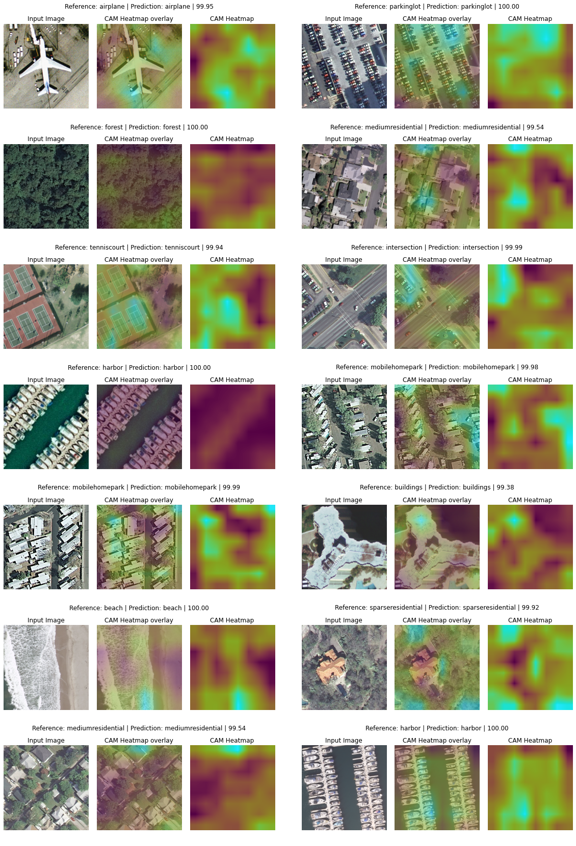
Key observations:

• For "harbor" images, the heatmap highlights the dock structures and boats — exactly the discriminative features for that class.
• For "runway" predictions, the model focuses on the long straight surfaces characteristic of airstrips.
• The heatmaps confirm that the model is looking at semantically meaningful regions, not artifacts or spurious correlations.

5. Understanding Feature Map Resolution

The class activation map at the last convolutional layer (block5_conv3) has the same spatial resolution as that layer's output. For VGG16 with 256×256 input, this is just 8×8 — each cell in the activation map represents a 32×32 pixel region of the original image:

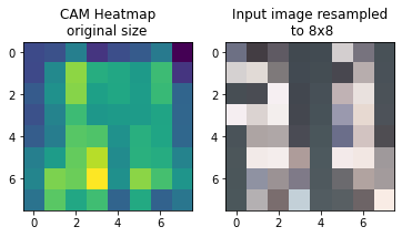
This coarse resolution explains why Grad-CAM heatmaps highlight broad regions rather than pixel-precise boundaries. The heatmap is bilinearly upscaled to match the input dimensions, but the spatial granularity is fundamentally limited by the convolutional layer's receptive field.

6. Multi-Layer Grad-CAM Analysis

We can compute Grad-CAM at any convolutional layer, not just the last one. Each layer captures features at a different level of abstraction:

• Early layers (block1, block2): Edges, corners, simple textures at high spatial resolution
• Middle layers (block3, block4): Parts of objects, complex textures
• Late layers (block5): Semantic concepts at low spatial resolution

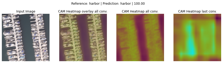
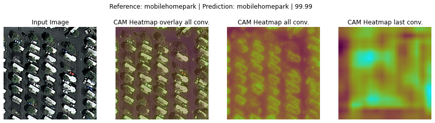
By averaging Grad-CAM heatmaps across all 13 convolutional layers, we obtain a more complete picture of the model's attention. Below we compare the averaged heatmap against the last-layer-only heatmap:

# Compute Grad-CAM for all convolutional layers
heatmaps = []
for layer in list_conv_layers:
    cam = GradCAM(model, id_class_pred, layer_name=layer)
    heatmaps.append(cam.compute_heatmap(x_i))

# Average all heatmaps for a holistic view
heatmap_avg = np.mean(np.array(heatmaps), axis=0).astype(np.uint8)

The all-layer average provides a more spatially detailed explanation, incorporating both the fine-grained attention of early layers and the semantic understanding of deeper layers.

7. Key Takeaways

1. Grad-CAM reveals the model's reasoning. It confirms that the CNN attends to semantically meaningful features (docks for harbors, runways for airports, vegetation patterns for agricultural land).
2. Use the Functional API for interpretability. The Sequential API wraps base models as single blocks, hiding individual layers. The Functional API exposes all layers, enabling per-layer analysis.
3. Heatmap resolution depends on the target layer. The last convolutional layer in VGG16 produces 8×8 activation maps for 256×256 inputs. Earlier layers offer higher spatial resolution but less semantic meaning.
4. Multi-layer averaging enriches explanations. Aggregating Grad-CAM across all convolutional layers provides both spatial detail and semantic relevance.
5. XAI builds trust in AI systems. Visualizing what a model "sees" helps domain experts validate predictions, identify failure modes, and ensure the model is learning the right features rather than dataset biases.

A model you cannot explain is a model you cannot trust. Grad-CAM bridges the gap between prediction accuracy and prediction understanding.