Working with Remote Sensing Data

Before training deep learning models on satellite imagery, we need to understand how remote sensing data is acquired, structured, and preprocessed. Unlike conventional RGB photographs, satellite images consist of multiple spectral bands, each capturing reflected electromagnetic radiation at a specific wavelength range. This multispectral richness opens the door to analyses far beyond what the human eye can perceive.

In this post, we walk through the fundamental operations of remote sensing data processing: reading and visualizing individual spectral bands, enhancing spatial resolution through pansharpening, and computing vegetation indices for land cover analysis. We use Landsat 8 imagery of Rio de Janeiro as our working example.

1. Image Acquisition Sources

Free, high-quality satellite imagery is available from multiple agencies worldwide. Knowing where to find the right data for your application is the first step in any remote sensing project:

• USGS Earth Explorer — Landsat, MODIS, DEMs, and more. The go-to portal for multi-decade Landsat archives.
• Copernicus Open Access Hub — Sentinel-1 (SAR), Sentinel-2 (multispectral), and Sentinel-3 missions from ESA.
• NASA Earthdata Search — A unified portal for NASA's Earth observation data across dozens of missions.
• DigitalGlobe Open Data Program — High-resolution commercial imagery released for disaster response and humanitarian efforts.

For this tutorial, we work with Landsat 8 OLI (Operational Land Imager) data, which provides 11 spectral bands ranging from coastal aerosol (0.43 μm) to thermal infrared (12.51 μm).

2. Spectral Band Visualization

Each Landsat 8 band captures a different slice of the electromagnetic spectrum, revealing different properties of the Earth's surface. We begin by loading all 8 bands of our Rio de Janeiro scene as individual GeoTIFF files:

import numpy as np
import tifffile
import cv2
from glob import glob
from os.path import join
from natsort import natsorted
import matplotlib.pyplot as plt

folder_images = "rj_image"
list_bands = glob(join(folder_images, "*.tif"))
list_bands = natsorted(list_bands, key=lambda y: y.lower())

Visualizing all 8 bands side by side immediately reveals how different wavelengths "see" the same landscape differently:

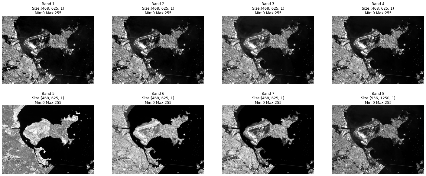
Notice how water bodies appear dark across most bands but vary in intensity. Vegetation is brighter in the Near-Infrared (Band 5) than in visible bands — this is because healthy vegetation strongly reflects NIR radiation, a property that forms the basis of vegetation indices we will explore later.

3. Pansharpening

Pansharpening is a fundamental image fusion technique that combines the high spatial resolution of the panchromatic band with the spectral richness of the multispectral bands. In Landsat 8, the multispectral bands have a 30-meter resolution, while the panchromatic band (Band 8) provides 15-meter resolution.

Landsat 8 Band Specifications

Band	Wavelength (μm)	Resolution (m)
Band 1 — Coastal aerosol	0.43–0.45	30
Band 2 — Blue	0.45–0.51	30
Band 3 — Green	0.53–0.59	30
Band 4 — Red	0.64–0.67	30
Band 5 — Near Infrared (NIR)	0.85–0.88	30
Band 6 — SWIR 1	1.57–1.65	30
Band 7 — SWIR 2	2.11–2.29	30
Band 8 — Panchromatic	0.50–0.68	15

We isolate the Red, Green, Blue, NIR, and Panchromatic bands for our fusion workflow:

red   = tifffile.imread(list_bands[3])   # Band 4 - Red
green = tifffile.imread(list_bands[2])   # Band 3 - Green
blue  = tifffile.imread(list_bands[1])   # Band 2 - Blue
nir   = tifffile.imread(list_bands[4])   # Band 5 - NIR
pan   = tifffile.imread(list_bands[7])   # Band 8 - Panchromatic

# Multispectral: (468, 625, 1) at 30m
# Panchromatic:  (936, 1250, 1) at 15m — exactly 2x the resolution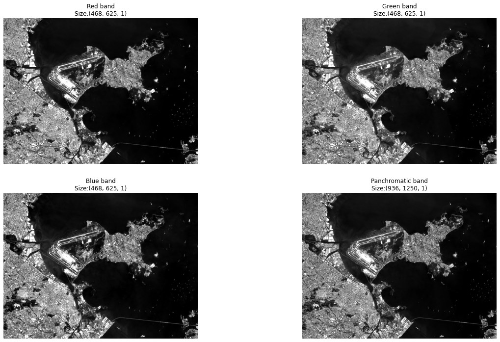

HSV Color Space Transformation

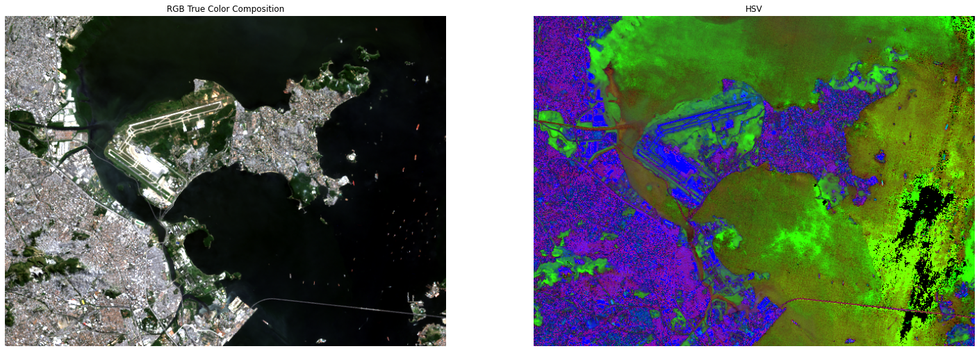
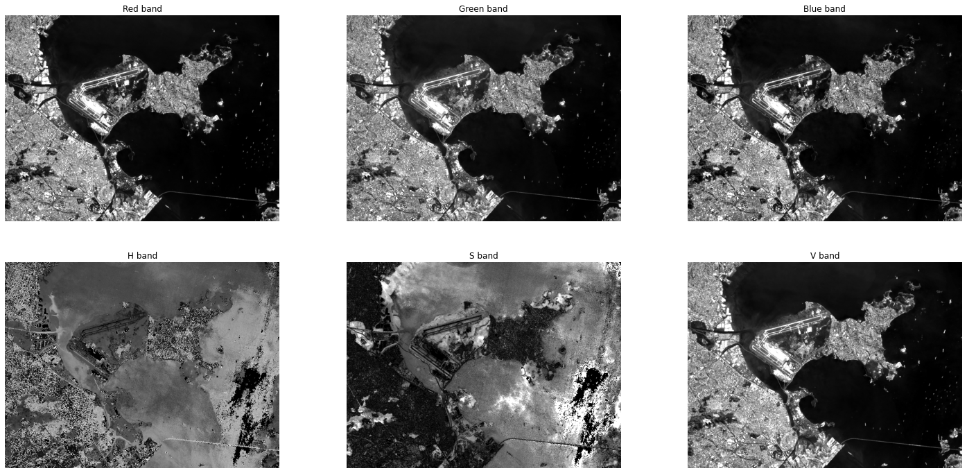
The pansharpening technique we employ is HSV band substitution. The key insight is that the HSV (Hue, Saturation, Value) color model separates chromatic information (Hue, Saturation) from luminance information (Value). Since the panchromatic band captures broadband intensity — essentially luminance at higher resolution — we can substitute it for the Value channel:

1. Compose the RGB true-color image from the multispectral bands
2. Convert RGB to HSV color space
3. Upscale the HSV image to match the panchromatic resolution
4. Replace the V (Value) channel with the panchromatic band
5. Convert back to RGB

# Compose RGB and convert to HSV
rgb = np.concatenate((red, green, blue), axis=2)
hsv = cv2.cvtColor(rgb, cv2.COLOR_RGB2HSV)

# Upscale HSV to panchromatic resolution and substitute Value channel
hsv_resized = cv2.resize(hsv, (pan.shape[1], pan.shape[0]))
hsv_resized[:, :, 2] = pan[:, :, 0]

# Convert back to RGB
pansharpened = cv2.cvtColor(hsv_resized, cv2.COLOR_HSV2RGB)

Below we compare the RGB and HSV representations. The decomposition into Hue, Saturation, and Value channels reveals how color and intensity information are separated:

Pansharpening Results

The result is striking. The pansharpened image retains the original color information from the multispectral bands while gaining the fine spatial detail from the panchromatic band. The improvement is most apparent in urban areas, where individual buildings and road networks become clearly distinguishable:

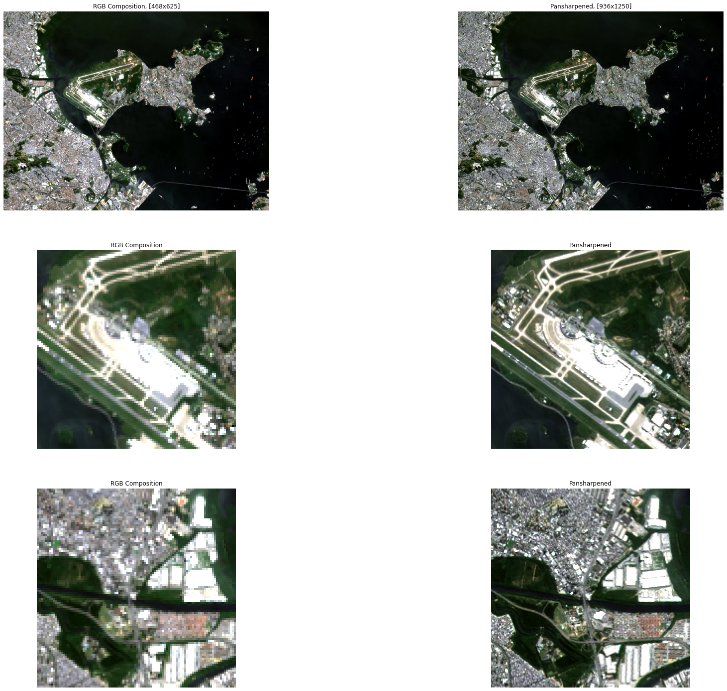
The original RGB composition at 468×625 pixels has been sharpened to 936×1250 pixels — a 4x increase in total pixel count. The zoomed insets clearly show the airport runways and coastal infrastructure rendered with significantly more detail in the pansharpened version.

4. Normalized Difference Vegetation Index (NDVI)

The NDVI is arguably the most widely used spectral index in remote sensing. It exploits the fact that healthy vegetation absorbs red light for photosynthesis while strongly reflecting near-infrared radiation. The index is computed as:

NDVI = (NIR − RED) / (NIR + RED)

NDVI values range from −1 to +1:

• Values near +1: Dense, healthy vegetation
• Values near 0: Bare soil, rock, or urban surfaces
• Negative values: Water bodies, clouds, or snow

We first visualize the four relevant bands (Red, Green, Blue, NIR) to understand the spectral contrast that NDVI leverages:

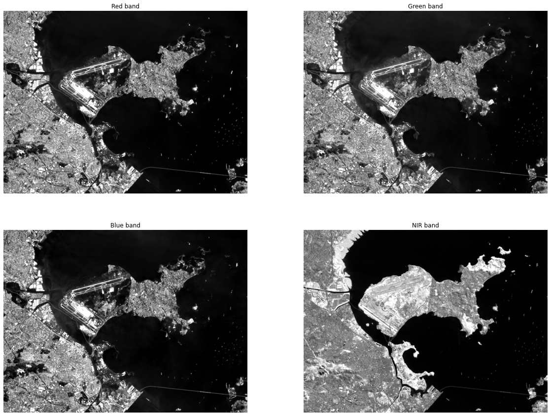
Computing NDVI is straightforward — note the cast to float to avoid integer overflow during subtraction:

ndvi = (nir.astype(float) - red.astype(float)) / \
       (nir.astype(float) + red.astype(float))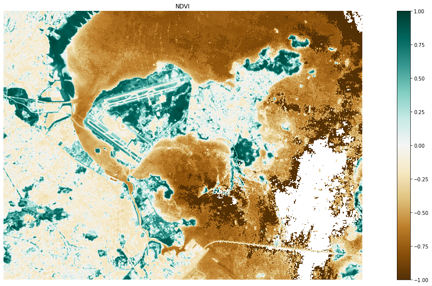

The NDVI map immediately reveals the spatial distribution of vegetation. The green/teal regions correspond to forested hillsides (including Tijuca National Park), while the brown/white areas indicate urban infrastructure and water bodies.

5. Vegetation Masking and Area Estimation

By thresholding the NDVI, we can create a binary vegetation mask and estimate the total vegetated area. Using an NDVI threshold of 0.5 (indicating moderately dense to dense vegetation):

rgb_veg = rgb.copy()
rgb_veg[np.squeeze(ndvi) < 0.5] = 0  # Mask non-vegetation pixels

# Calculate area: each pixel = 30m x 30m
non_zero = np.sum(rgb_veg[:, :, 0] != 0)
total_area = non_zero * 30 * 30 * 1e-6
print(f"Vegetation area: {total_area} km²")
# Output: Vegetation area: 25.4988 km²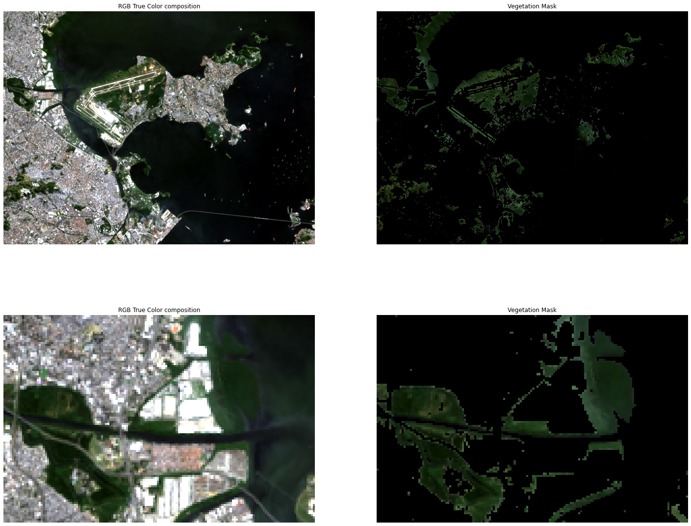

The vegetation mask cleanly isolates forested areas while suppressing urban structures, water, and bare soil. The computed vegetation area of 25.50 km² provides a quantitative measure that can be tracked over time for deforestation monitoring or urban growth analysis.

6. Key Takeaways

1. Multispectral data is rich: Each spectral band captures different surface properties. Understanding these differences is essential before applying any machine learning pipeline.
2. Pansharpening doubles spatial detail: The HSV band substitution method is simple yet effective. More advanced methods (Brovey transform, PCA-based fusion, wavelet fusion) can yield even better results.
3. NDVI is a powerful baseline: Despite its simplicity, NDVI remains one of the most reliable indicators for vegetation monitoring, agriculture assessment, and environmental change detection.
4. Preprocessing matters: Casting data types, handling nodata values, and understanding band specifications are not glamorous tasks, but they directly affect the quality of any downstream analysis or model training.
5. Free data is abundant: Multiple space agencies provide open-access satellite data. For deep learning applications, this means virtually unlimited training data for Earth observation tasks.