Semantic Segmentation with U-Net on Aerial Imagery
Unlike image classification, which assigns a single label to an entire image, semantic segmentation assigns a class label to every pixel. This is essential in remote sensing, where a single aerial image may contain buildings, roads, vegetation, and vehicles — all of which must be delineated precisely.
In this post, we implement U-Net — the canonical encoder-decoder architecture with skip connections — for multi-class semantic segmentation on the ISPRS Vaihingen aerial imagery dataset. The model achieves 82.06% test accuracy with a mean IoU of 0.552 across six land-cover classes.
1. The ISPRS Vaihingen Dataset
The ISPRS 2D Semantic Labeling — Vaihingen dataset is a widely used benchmark for urban scene understanding from aerial imagery. It consists of 33 image patches of varying sizes, each containing:
- True Orthophoto (TOP) — False-color RGB composite (near-infrared, red, green) at 9 cm ground sampling distance
- Digital Surface Model (DSM) — Height information for each pixel
- Ground Truth — Pixel-wise annotations for 6 semantic classes
The six classes and their color codes are:
| Class | Color | RGB |
|---|---|---|
| Impervious surfaces | (255, 255, 255) | |
| Building | (0, 0, 255) | |
| Low vegetation | (0, 255, 255) | |
| Tree | (0, 255, 0) | |
| Car | (255, 255, 0) | |
| Clutter/background | (255, 0, 0) |
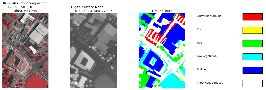
A sample patch from the Vaihingen dataset: false-color RGB composite, Digital Surface Model, ground truth annotations, and the class color legend.
Following the benchmark guidelines, we split the 33 patches into 16 training and 17 test areas. From the training set, 25% is reserved for validation (4 patches), leaving 12 patches for training.
2. Custom Data Generator for Patch Extraction
The Vaihingen images are large (up to 3000×3000 pixels), far too big to feed directly into a CNN. We extract fixed-size 256×256 patches using a sliding window with a configurable stride. This is implemented as a custom Keras Sequence data generator that:
- Pre-computes all valid (image_path, coordinate) pairs across all images
- Loads only the required patch region using PIL's lazy loading and
crop() - Converts RGB ground truth masks to integer class indices using a color-to-index mapping
- Returns one-hot encoded labels for categorical cross-entropy training
class DataGenerator(keras.utils.Sequence):
    def __init__(self, batch_size, patch_size, step_size,
                 list_top, list_gts, n_classes,
                 colormap_gt=None, shuffle=True):
        self.batch_size = batch_size
        self.patch_size = patch_size
        self.step_size = step_size
        self.list_top = list_top
        self.list_gts = list_gts
        self.n_classes = n_classes
        self.colormap_gt = colormap_gt
        self.shuffle = shuffle
        self.path_coords = self.__get_path_coords()
        self.n_patchs = len(self.path_coords)

    def __get_path_coords(self):
        path_coords = []
        for path_image, path_label in zip(self.list_top, self.list_gts):
            width, height = Image.open(path_label).size
            for y in range(0, height, self.step_size):
                for x in range(0, width, self.step_size):
                    if (x + self.patch_size) > width:
                        x = width - self.patch_size
                    if (y + self.patch_size) > height:
                        y = height - self.patch_size
                    path_coords.append((path_image, path_label, (x, y)))
        return path_coords
A key optimization is using Pillow's lazy loading: Image.open() reads only the file header, and crop() loads only the requested region into memory. This is critical when working with large geospatial images that may not fit entirely in RAM.
# Efficient patch extraction with PIL
data = Image.open(path)
data = data.crop((x, y, x + patch_size, y + patch_size))
data = np.asarray(data)  # only the cropped area is loaded
The ground truth conversion maps each RGB color to an integer class index:
color2index = {
    (255, 255, 255): 0,  # Impervious surfaces
    (0,   0,   255): 1,  # Building
    (0,   255, 255): 2,  # Low vegetation
    (0,   255, 0  ): 3,  # Tree
    (255, 255, 0  ): 4,  # Car
    (255, 0,   0  ): 5   # Clutter/background
}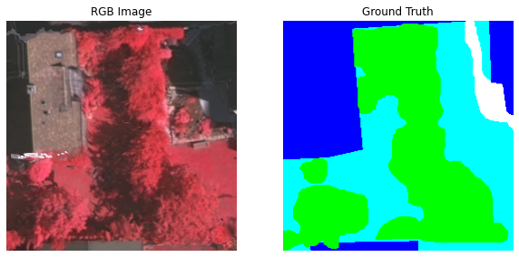
An extracted 256×256 patch and its corresponding ground truth mask, produced by the DataGenerator.
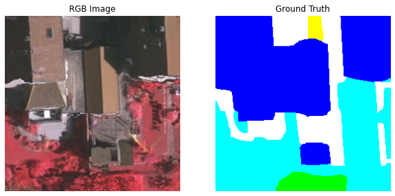
Another patch pair from the training set, showing the diversity of urban structures in the Vaihingen dataset.
With batch_size=8, patch_size=256, and step_size=256, the generator produces 128 training batches and 38 validation batches per epoch.
3. U-Net Architecture
U-Net was originally proposed for biomedical image segmentation and has since become the de facto standard for many segmentation tasks. Its defining feature is the symmetric encoder-decoder structure with skip connections that concatenate feature maps from the encoder to the decoder at each resolution level.
Our implementation uses three building blocks:
- Conv Block — Two consecutive 3×3 convolutions with ReLU activation and He normal initialization
- Downsampling — Conv block followed by 2×2 max pooling and 30% dropout
- Upsampling — 3×3 transposed convolution (stride 2), concatenation with the skip connection, dropout, and a conv block
def conv_block(x, n_filters, times=2):
    for i in range(times):
        x = Conv2D(filters=n_filters, kernel_size=3, strides=1,
                   padding="same", activation="relu",
                   kernel_initializer="he_normal")(x)
    return x

def downsampling(x, n_filters, times=2):
    feat = conv_block(x, n_filters, times=times)
    pool = MaxPooling2D(pool_size=2)(feat)
    pool = Dropout(rate=0.3)(pool)
    return feat, pool

def upsampling(input, filters, layer_concat=None):
    x = Conv2DTranspose(filters=filters, kernel_size=3,
                        strides=2, padding="same")(input)
    if layer_concat is not None:
        x = concatenate([x, layer_concat])
    x = Dropout(rate=0.3)(x)
    x = conv_block(x, filters, times=2)
    return x
The full U-Net is assembled using the Functional API:
def get_unet(img_size, n_classes):
    input = Input(shape=(img_size, img_size, 3))
    # Encoder
    f1, p1 = downsampling(input, 64, times=2)
    f2, p2 = downsampling(p1, 128, times=2)
    f3, p3 = downsampling(p2, 256, times=2)
    # Bottleneck
    bottleneck = conv_block(p3, 512, times=2)
    # Decoder
    u7 = upsampling(bottleneck, 256, layer_concat=f3)
    u8 = upsampling(u7, 128, layer_concat=f2)
    u9 = upsampling(u8, 64, layer_concat=f1)
    # Output
    output = Conv2D(filters=n_classes, kernel_size=1,
                    padding="same", activation="softmax")(u9)
    return Model(inputs=input, outputs=output, name="UNet")
The resulting model has 8,557,830 trainable parameters. Note that we use a bottleneck of 512 filters rather than the original paper's 1024, which reduces memory usage while still providing sufficient capacity for this dataset.
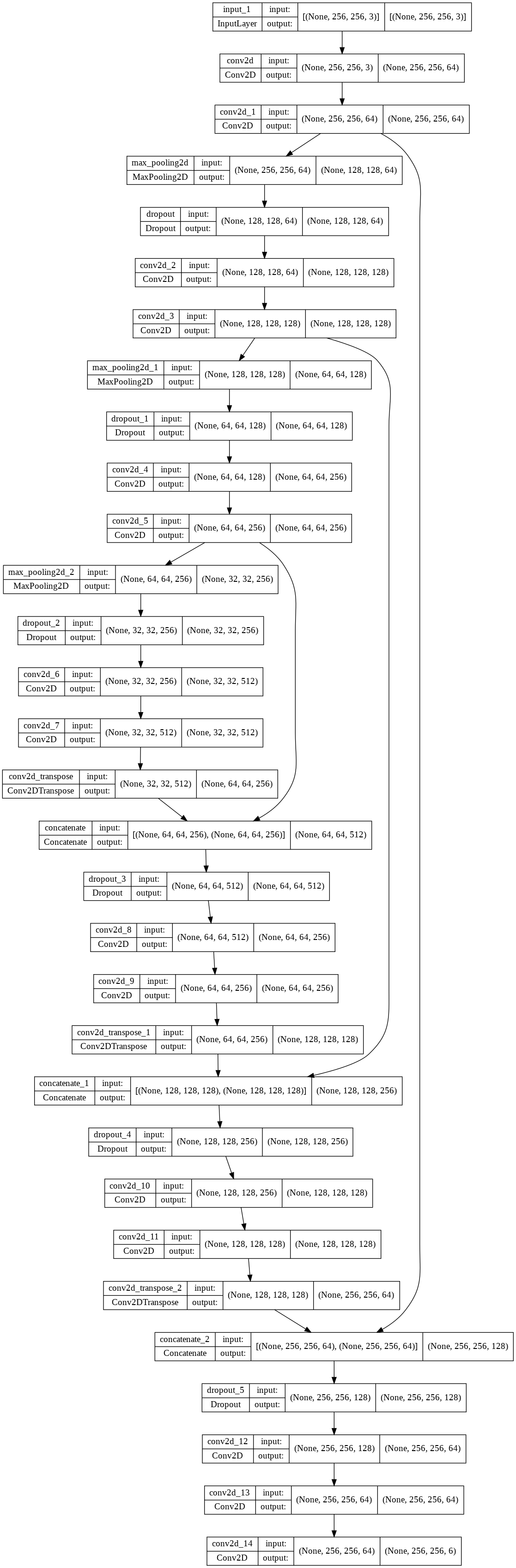
The U-Net architecture: three downsampling stages (64 → 128 → 256), a 512-filter bottleneck, and three upsampling stages with skip connections restoring spatial resolution.
4. Training Configuration
We train with the Adam optimizer and categorical cross-entropy loss. The key metric is Mean Intersection over Union (mIoU), which is the standard evaluation metric for semantic segmentation:
IoU = TP / (TP + FP + FN)
where TP, FP, and FN are the true positives, false positives, and false negatives for each class. Mean IoU averages across all classes, giving equal weight to minority classes like "car" and "clutter."
model_unet.compile(
    optimizer=Adam(),
    loss="categorical_crossentropy",
    metrics=["accuracy",
             OneHotMeanIoU(num_classes=n_classes, name="iou")]
)
Two callbacks govern training:
- ModelCheckpoint — Saves the best model based on validation IoU
- EarlyStopping — Stops training after 30 epochs without improvement
autosave_unet = ModelCheckpoint("segmentation_unet.h5",
                                mode="max",
                                save_best_only=True,
                                monitor="val_iou",
                                verbose=1)

early_stopping = EarlyStopping(patience=30, verbose=1, mode='auto')

history_unet = model_unet.fit(data_gen_train,
                              epochs=200,
                              validation_data=data_gen_val,
                              callbacks=[autosave_unet, early_stopping],
                              workers=4,
                              use_multiprocessing=True,
                              max_queue_size=20)
5. Results
After training, we evaluate the model on all three splits:
| Split | Loss | Accuracy | Mean IoU |
|---|---|---|---|
| Train | 0.2185 | 91.83% | 0.730 |
| Validation | 0.7123 | 83.14% | 0.551 |
| Test | 0.6403 | 82.06% | 0.552 |
The gap between training and validation/test performance suggests some overfitting, which is expected given the relatively small number of training patches (12 images). The consistent validation and test IoU (~0.55) indicates good generalization within the expected capacity of this model configuration.
6. Prediction Visualizations
Below we visualize model predictions on test patches alongside the input RGB image, the ground truth reference, and per-class IoU scores:
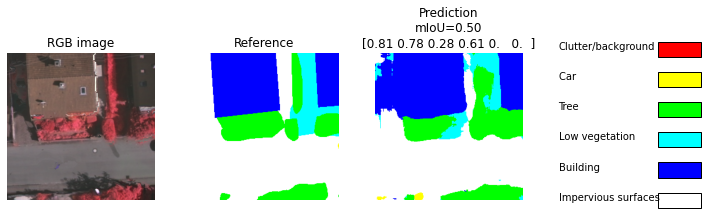
Test patch prediction with per-class IoU breakdown. The model correctly delineates major structures like buildings and vegetation.
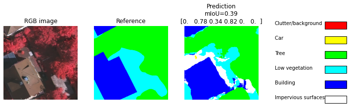
Another test prediction demonstrating the model's ability to segment different land cover types at the pixel level.
Key observations from the predictions:
- Buildings and trees are generally well-segmented, as these classes have strong spectral and spatial signatures in the false-color imagery
- Impervious surfaces vs. low vegetation boundaries can be noisy, as these classes sometimes share similar spectral characteristics
- Cars are the most challenging class due to their small size relative to the 256×256 patch, resulting in class imbalance
- Skip connections are crucial for recovering fine-grained spatial detail that would otherwise be lost through the pooling operations
7. Key Takeaways
- U-Net excels at dense prediction tasks. The encoder-decoder architecture with skip connections effectively combines high-level semantic features with low-level spatial details, making it well-suited for segmentation.
- Custom data generators are essential for large imagery. Geospatial images are often too large to fit in memory. Patch-based generators with PIL's lazy loading allow efficient training on any image size.
- Mean IoU is the right metric. Pixel accuracy can be misleading when classes are imbalanced. Mean IoU provides a fairer assessment by treating all classes equally, highlighting weaknesses on minority classes like cars.
- The gap between training and test IoU (0.73 vs 0.55) suggests room for improvement through data augmentation, deeper architectures, or incorporating the DSM as an additional input channel.
- Patch size and stride affect both performance and training time. A stride equal to the patch size (256) provides non-overlapping patches; overlapping extraction (smaller stride) would increase the training set at the cost of longer epochs.
Semantic segmentation transforms aerial imagery from visual data into actionable maps. U-Net's elegant architecture — compress, then expand with memory — remains a powerful baseline for any pixel-wise classification task.