Single-Class Object Localization with VGG16
Object detection is often introduced as a complex, multi-stage pipeline involving region proposals, non-maximum suppression, and anchor boxes. But before tackling all of that, it is instructive to solve the simplest case: single-class object localization — predicting the bounding box coordinates of a single known object in each image.
In this post, we frame localization as a regression problem. Using a frozen VGG16 backbone and a small fully-connected head, we train a model to predict bounding box coordinates for airplanes in the Caltech101 dataset. This approach strips object detection down to its essential components: feature extraction and coordinate regression.
1. The Caltech101 Dataset
The Caltech101 dataset contains images of objects belonging to 101 categories. For this single-class localization task, we use only the airplanes category: approximately 800 images, each roughly 300×200 pixels, with bounding box annotations provided as CSV files.
Each annotation consists of four normalized coordinates: (x1, y1, x2, y2) representing the top-left and bottom-right corners of the bounding box. The coordinates are normalized to the [0, 1] range relative to the image dimensions, which is essential since VGG16 expects a fixed 224×224 input.
class_name = 'airplanes'
annotations_file = os.path.join(BOXES_PATH, class_name + ".csv")
annotations = pd.read_csv(annotations_file)

# Bounding box coordinates
bbox_cols = ['x1', 'y1', 'x2', 'y2']
annotations['BBox'] = [x for x in
    annotations[bbox_cols].to_numpy().astype(np.int64)]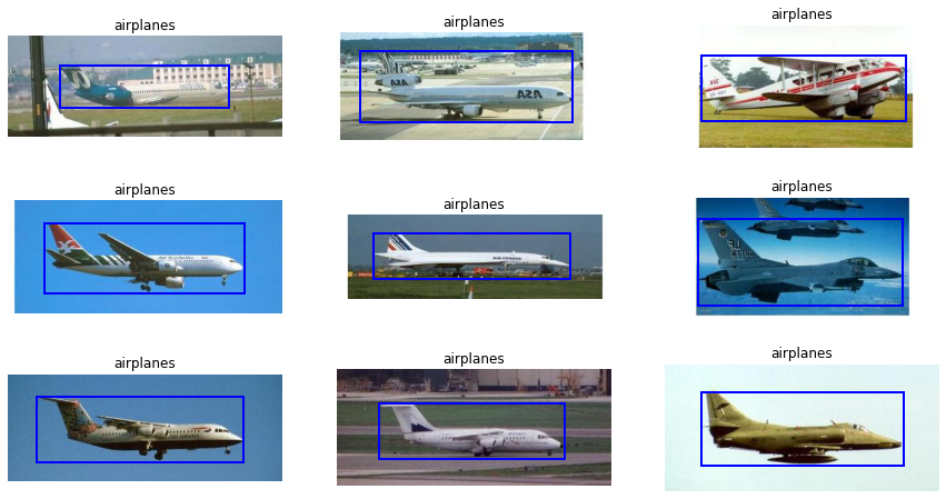
Training samples from the airplanes category with ground truth bounding boxes (red) overlaid on the original images.
2. Data Preparation
Since VGG16 requires 224×224 input images, all images and their bounding boxes must be resized accordingly. The bounding box coordinates are normalized to the [0, 1] range so they remain valid regardless of the input resolution:
MODEL_INPUT_SIZE = (224, 224)

# For each image:
# 1. Get original dimensions
w, h = imagesize.get(image_path)

# 2. Normalize bounding box to [0, 1]
startX = bbox[0] / w
startY = bbox[1] / h
endX   = bbox[2] / w
endY   = bbox[3] / h

# 3. Resize image to 224x224
image = load_img(image_path, target_size=MODEL_INPUT_SIZE)
image = img_to_array(image)
The dataset is split into training, validation, and test sets using scikit-learn's train_test_split:
from sklearn.model_selection import train_test_split

# 80% train, 10% validation, 10% test
trainImages, testImages, trainTargets, testTargets = \
    train_test_split(data, targets, test_size=0.2, random_state=seed)

trainImages, valImages, trainTargets, valTargets = \
    train_test_split(trainImages, trainTargets, test_size=0.125,
                     random_state=seed)
3. Model Architecture
The key insight is that localization can be treated as a regression task: instead of predicting class probabilities, we predict four continuous values (the bounding box coordinates). The architecture consists of:
- VGG16 backbone (frozen) — Pre-trained on ImageNet, used purely as a feature extractor. All convolutional weights are frozen to prevent overfitting on the small dataset.
- Flatten layer — Converts the 7×7×512 feature map to a 1D vector
- FC regression head — Three dense layers (128 → 64 → 32 → 4) with ReLU activations, outputting 4 sigmoid-activated values representing the normalized bounding box coordinates
# Load VGG16 without the classification head
vgg = VGG16(weights="imagenet", include_top=False,
            input_tensor=Input(shape=(224, 224, 3)))
vgg.trainable = False  # freeze all layers

# Flatten VGG output
flatten = Flatten()(vgg.output)

# Regression head for bounding box prediction
bboxHead = Dense(128, activation="relu")(flatten)
bboxHead = Dense(64, activation="relu")(bboxHead)
bboxHead = Dense(32, activation="relu")(bboxHead)
bboxHead = Dense(4, activation="sigmoid")(bboxHead)

model = Model(inputs=vgg.input, outputs=bboxHead)
The final layer uses sigmoid activation because the bounding box coordinates are normalized to [0, 1]. The loss function is mean squared error (MSE), which directly penalizes the Euclidean distance between predicted and ground truth coordinates:
INIT_LR = 1e-4
NUM_EPOCHS = 25
BATCH_SIZE = 16

opt = Adam(learning_rate=INIT_LR)
model.compile(loss="mse", optimizer=opt)
4. Training
The model is trained for 25 epochs with a batch size of 16. Since VGG16 features are frozen, only the regression head (~2M parameters) is being optimized. This makes training fast and reduces the risk of overfitting:
H = model.fit(trainImages, trainTargets,
              validation_data=(valImages, valTargets),
              batch_size=BATCH_SIZE,
              epochs=NUM_EPOCHS,
              callbacks=[tensorboard_callback, callback_checkpoint],
              verbose=1)
5. Results and Predictions
After training, the model predicts bounding box coordinates on unseen test images. Predictions (green boxes) are compared against ground truth annotations (red boxes):
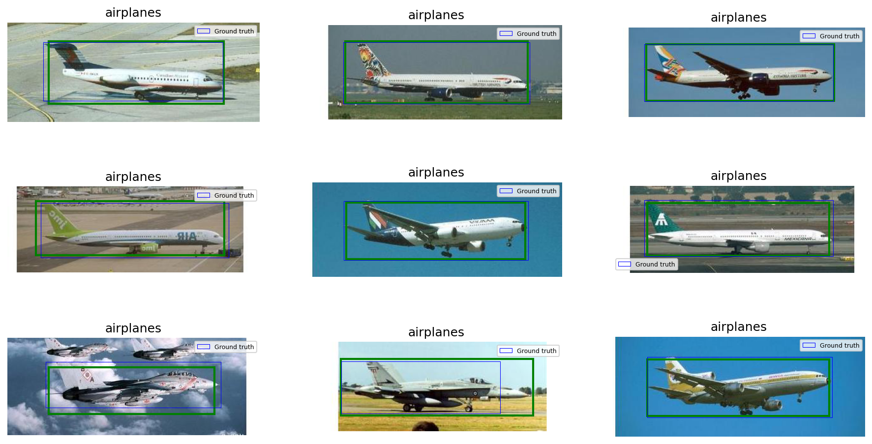
Test set predictions: green boxes show the model's predicted bounding boxes, red boxes show the ground truth. The model achieves tight localization on most samples.
To understand failure modes, we also visualize the worst predictions — the test samples with the largest coordinate error:
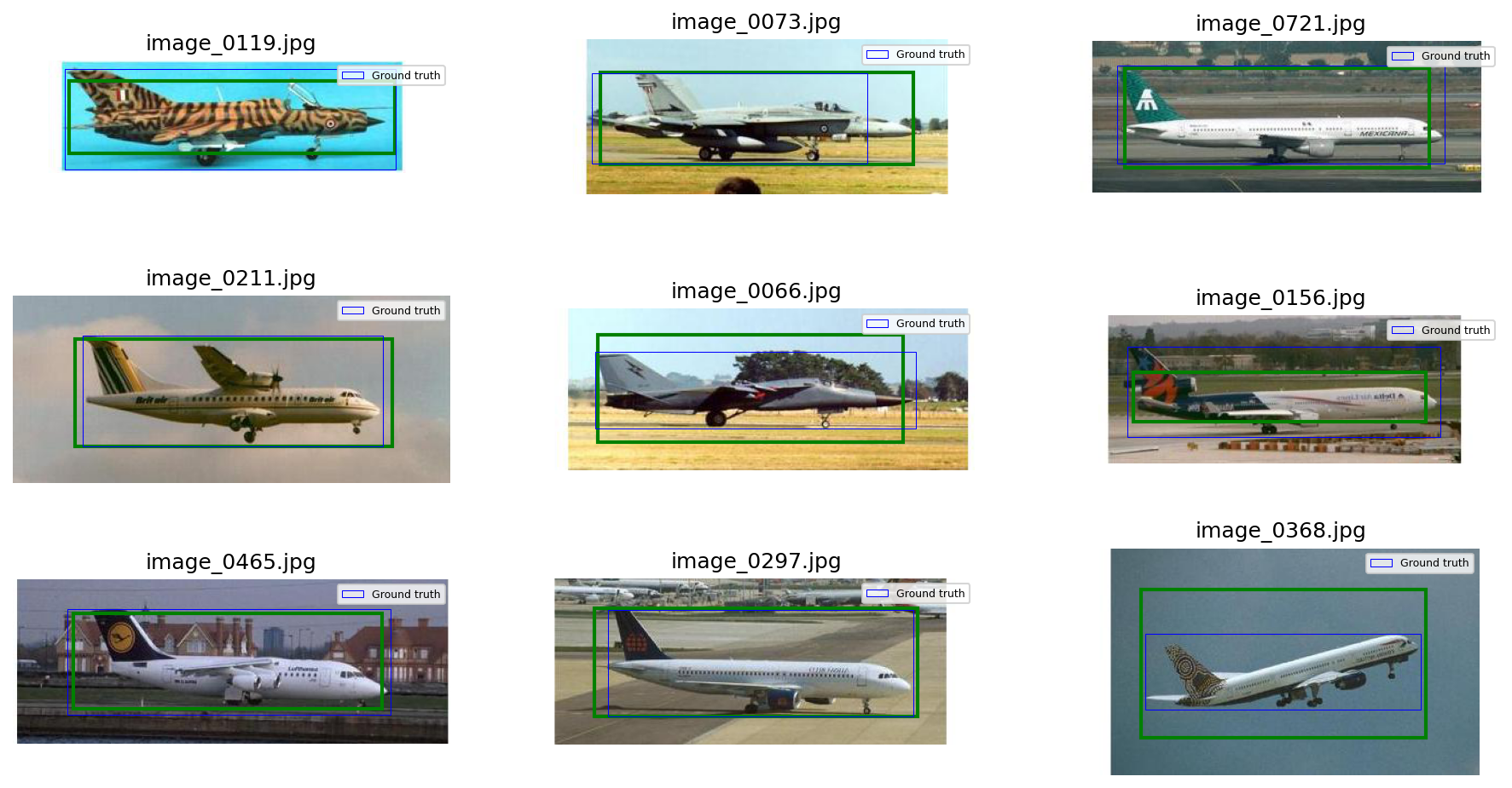
The 9 worst test predictions ranked by absolute coordinate error. Failures tend to occur on unusual viewpoints, partially occluded aircraft, or images with multiple objects.
6. Key Takeaways
- Object localization is regression. By framing bounding box prediction as a regression task with MSE loss, we bypass the complexity of region proposals and anchor-based methods entirely. For single-class, single-object scenarios, this is sufficient.
- Transfer learning makes small datasets viable. With only ~800 images, training a CNN from scratch would likely fail. VGG16's pre-trained features provide a rich representation that a small regression head can leverage effectively.
- Sigmoid output + normalized coordinates is a clean design. Normalizing bounding boxes to [0, 1] and using sigmoid activation ensures predictions are always valid coordinates, regardless of the original image size.
- Failure cases reveal limitations. The worst predictions occur on atypical images — unusual viewpoints, occlusions, or multiple objects. This highlights why full object detection frameworks (like YOLO or Faster R-CNN) are needed for real-world scenarios.
- This is a stepping stone to full detection. The concepts here — feature extraction, bounding box regression, coordinate normalization — are fundamental building blocks of modern object detection architectures.
Before learning to detect many objects in complex scenes, learn to find one. Single-class localization strips detection to its essence: extract features, regress coordinates, evaluate predictions.