Multi-Class Object Detection with a Custom Data Generator
In the previous post, we built a single-class localizer that predicts bounding boxes for one object type. The natural next step is multi-class object detection: simultaneously predicting what the object is and where it is in the image.
This requires a multi-output model with two heads: a classification branch that predicts the object category, and a regression branch that predicts the bounding box coordinates. We implement this using VGG16 transfer learning on the Caltech101 dataset, achieving 99.56% classification accuracy and 88.24% bounding box accuracy on the test set.
1. Dataset and Class Selection
The Caltech101 dataset contains 101 object categories with bounding box annotations. For this experiment, we select 6 visually distinct classes:
- Airplanes
- Motorbikes
- Faces
- Helicopters
- Cameras
- Car (side view)
class_names = ['airplanes', 'Motorbikes', 'Faces',
               'helicopter', 'camera', 'car_side']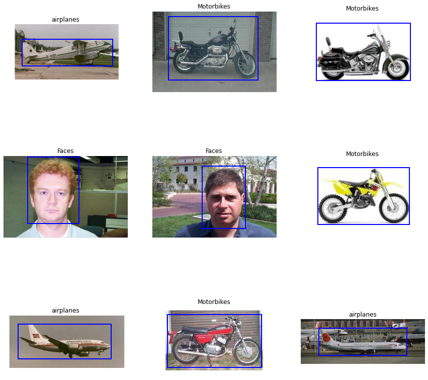
Samples from the six selected classes with ground truth bounding boxes overlaid. Each class has distinct visual characteristics.
Bounding box coordinates are normalized to the [0, 1] range relative to image dimensions, ensuring consistency when images are resized to 224×224 for VGG16:
# Normalize bounding box coordinates to [0, 1]
BBoxes_normalized = []
for idx, row in df2.iterrows():
    w, h = row['w_image'], row['h_image']
    bbox = row['BBox']
    BBoxes_normalized.append([
        bbox[0] / w,  # x1
        bbox[1] / h,  # y1
        bbox[2] / w,  # x2
        bbox[3] / h   # y2
    ])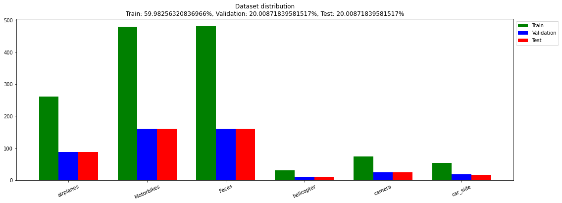
Distribution of samples across the six classes in training, validation, and test splits.
2. Custom Data Generator
With thousands of images across multiple classes, loading everything into memory is impractical. We implement a custom tf.keras.utils.Sequence data generator that:
- Loads images on-the-fly from disk in batches
- Resizes images to the model's input size (224×224)
- Applies optional preprocessing (e.g., VGG16's
preprocess_input) - Returns both classification labels (one-hot) and bounding box coordinates
class CustomDataGenerator(tf.keras.utils.Sequence):
    def __init__(self, path_images, labels, BBoxes,
                 n_classes, out_size=(224, 224, 3),
                 batch_size=16, preprocess_input=None,
                 convert_to_one_hot=True, shuffle=True):
        self.path_images = path_images
        self.labels = labels
        self.BBoxes = BBoxes
        self.n_classes = n_classes
        self.out_size = out_size
        self.batch_size = batch_size
        self.preprocess_input = preprocess_input
        self.convert_to_one_hot = convert_to_one_hot
        self.shuffle = shuffle

    def __len__(self):
        return int(np.ceil(len(self.path_images) / self.batch_size))

    def __getitem__(self, idx):
        batch_paths = self.path_images[idx*self.batch_size:
                                        (idx+1)*self.batch_size]
        # Load and preprocess images
        images = images_resize(batch_paths, self.out_size[:2])
        if self.preprocess_input:
            images = self.preprocess_input(images)
        # Get corresponding labels and bounding boxes
        labels = self.labels[idx*self.batch_size:
                             (idx+1)*self.batch_size]
        bboxes = self.BBoxes[idx*self.batch_size:
                             (idx+1)*self.batch_size]
        if self.convert_to_one_hot:
            labels = to_categorical(labels, self.n_classes)
        return images, {"label": labels, "BBox": bboxes}
The generator returns a dictionary of outputs matching the model's two output heads, enabling Keras to route the correct targets to each loss function.
3. Multi-Output Model Architecture
The model extends the single-class localizer with a dual-head architecture. Both heads share the same frozen VGG16 backbone, but diverge into separate fully-connected paths:
- Classification head (
softmaxHead) — 512 → 512 → Nclasses with dropout (0.5) and softmax activation - Regression head (
bboxHead) — 128 → 64 → 32 → 4 with sigmoid activation for normalized coordinates
# Frozen VGG16 backbone
vgg = VGG16(weights="imagenet", include_top=False,
            input_tensor=Input(shape=(224, 224, 3)))
vgg.trainable = False
flatten = Flatten()(vgg.output)

# Classification head
softmaxHead = Dense(512, activation="relu")(flatten)
softmaxHead = Dropout(0.5)(softmaxHead)
softmaxHead = Dense(512, activation="relu")(softmaxHead)
softmaxHead = Dropout(0.5)(softmaxHead)
softmaxHead = Dense(num_classes, activation="softmax",
                    name="label")(softmaxHead)

# Regression head
bboxHead = Dense(128, activation="relu")(flatten)
bboxHead = Dense(64, activation="relu")(bboxHead)
bboxHead = Dense(32, activation="relu")(bboxHead)
bboxHead = Dense(4, activation="sigmoid",
                 name="BBox")(bboxHead)

# Combined model
model = Model(inputs=vgg.input,
              outputs=(softmaxHead, bboxHead))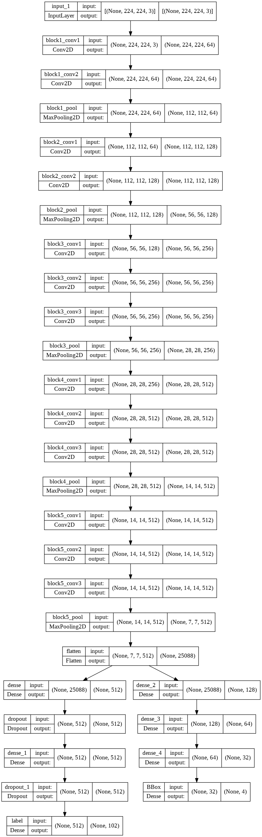
The dual-head architecture: a shared VGG16 backbone feeds into separate classification (softmax) and localization (sigmoid) branches.
4. Multi-Task Loss
Training a multi-output model requires defining separate losses for each head and combining them. We use categorical cross-entropy for classification and MSE for bounding box regression:
# Separate losses for each output
losses = {
    "label": "categorical_crossentropy",
    "BBox": "mean_squared_error"
}

# Equal weighting (can be tuned)
lossWeights = {
    "label": 1.0,
    "BBox": 1.0
}

opt = Adam(learning_rate=1e-4)
model.compile(loss=losses, optimizer=opt,
              metrics=["accuracy"],
              loss_weights=lossWeights)
The loss_weights dictionary controls the relative importance of each task. With equal weights (1.0 each), both tasks contribute equally to the gradient updates. In practice, tuning these weights can improve results when one task is more difficult than the other.
5. Training
The model is trained for up to 200 epochs with early stopping (patience of 50 epochs):
H = model.fit(train_data_gen,
              validation_data=val_data_gen,
              epochs=200,
              callbacks=[tensorboard_callback,
                         callback_checkpoint,
                         early_stopping],
              verbose=1)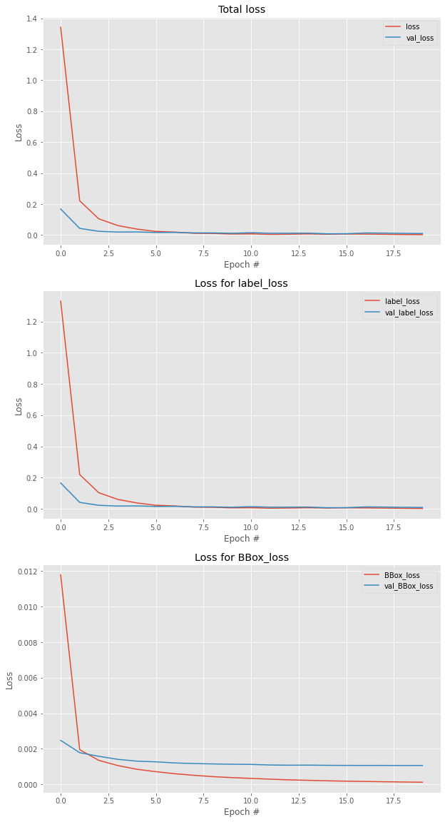
Training curves showing total loss, classification loss, and bounding box regression loss over epochs.
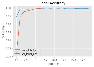
Classification accuracy convergence during training for both the training and validation sets.
6. Results
On the test set, the model achieves:
| Metric | Test Score |
|---|---|
| Classification accuracy | 99.56% |
| Bounding box accuracy | 88.24% |
| Total loss | 0.0130 |
| Label loss | 0.0120 |
| BBox loss | 0.0011 |
The near-perfect classification accuracy (99.56%) demonstrates that VGG16 features are highly discriminative for these six visually distinct classes. The bounding box regression also performs well, with an MSE loss of only 0.0011 on normalized coordinates.
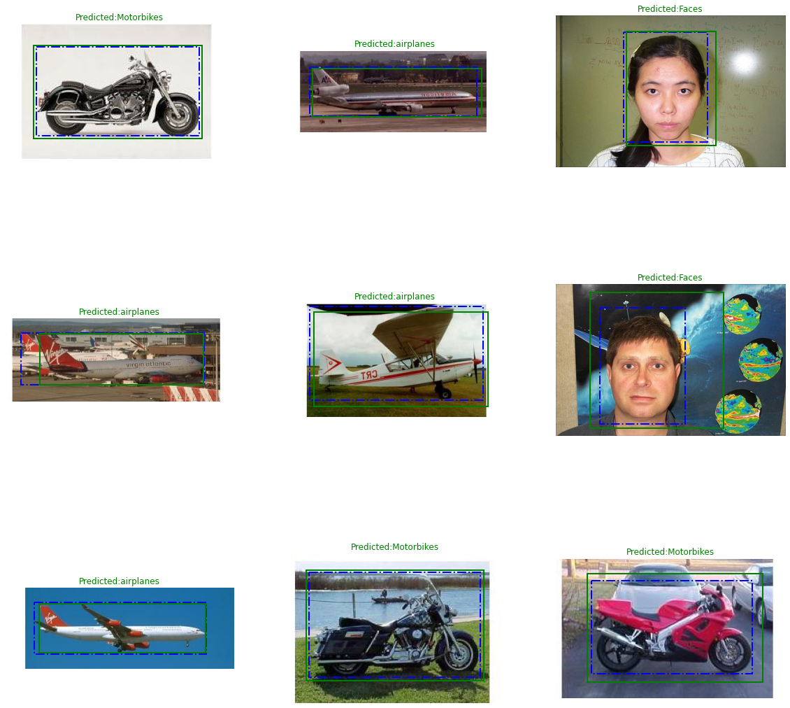
Test set predictions with predicted bounding boxes (green) and ground truth (red). The model correctly classifies and localizes objects across all six categories.
7. Limitations
While the results are impressive, this approach has fundamental limitations that motivate the use of dedicated detection frameworks like YOLO or Faster R-CNN:
- Single object per image. The model predicts exactly one bounding box and one class label. Images with multiple objects will only detect the most confident one.
- Fixed number of classes. Adding new classes requires retraining the entire classification head.
- No scale invariance. The model processes the entire image at a single scale, unlike modern detectors that use feature pyramids.
- No non-maximum suppression. Since only one box is predicted, there is no mechanism to handle overlapping detections.
8. Key Takeaways
- Multi-task learning is natural for detection. By sharing a backbone and training classification and regression jointly, the model learns features that serve both tasks. This shared representation is more efficient than training separate models.
- Custom data generators enable scalable training. Loading images on-the-fly with batch processing and optional preprocessing allows training on datasets that exceed available memory.
- Output naming enables clean multi-loss training. Keras' named outputs (
name="label",name="BBox") allow defining per-head losses and metrics through dictionaries, making the training configuration readable and maintainable. - Loss weighting is a design decision. Equal weights work well here because both tasks converge at similar rates. For harder problems, tuning the ratio between classification and regression loss can significantly affect performance.
- This is the foundation for modern detectors. YOLO, SSD, and Faster R-CNN all build on these same principles — shared feature extraction, multi-task loss, and bounding box regression — but add region proposals, anchor boxes, and multi-scale processing to handle real-world complexity.
Multi-class object detection is fundamentally two problems solved simultaneously: "what is it?" and "where is it?" The dual-head architecture makes this explicit, and the shared backbone ensures both answers are grounded in the same visual understanding.