DeepLabV3+ vs U-Net: Advanced Semantic Segmentation
In the previous post, we implemented a basic U-Net for semantic segmentation on the ISPRS Vaihingen dataset. While the results were promising, there is significant room for improvement. In this post, we explore three strategies to push segmentation quality further:
- Data augmentation with Albumentations to increase training data diversity
- DeepLabV3+ — a state-of-the-art architecture using atrous convolutions and a ResNet50 backbone
- Focal loss — a loss function designed to handle class imbalance
We compare four model configurations and find that DeepLabV3+ with augmentation achieves the best test mIoU of 0.643, a substantial improvement over the baseline U-Net (0.454).
1. Dataset Recap
We use the same ISPRS Vaihingen dataset as before: 33 aerial image patches with 6 semantic classes (impervious surfaces, building, low vegetation, tree, car, clutter). The data split follows the benchmark guidelines with 12 training, 4 validation, and 17 test patches.
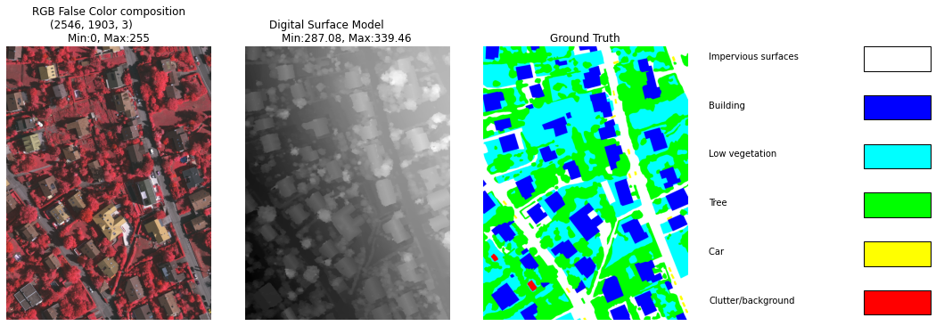
A patch from the Vaihingen dataset: false-color RGB, Digital Surface Model, ground truth, and class color legend.
2. Data Augmentation with Albumentations
The limited number of training patches (12 images) makes the model prone to overfitting. Data augmentation artificially increases training diversity by applying random geometric and photometric transformations to each patch during training.
We use Albumentations, a fast image augmentation library that consistently applies the same transformation to both the input image and its segmentation mask:
from albumentations import (Compose, HorizontalFlip, VerticalFlip,
                            RandomRotate90, ShiftScaleRotate)

def augmentation():
    return Compose([
        HorizontalFlip(p=0.5),
        VerticalFlip(p=0.5),
        RandomRotate90(p=0.5),
        ShiftScaleRotate(shift_limit=0.01,
                         scale_limit=0,
                         rotate_limit=5, p=0.5),
    ], is_check_shapes=False)
Each augmentation is applied with a probability p, creating a combinatorial explosion of training variations from the same source patches. Crucially, the mask is transformed identically to the image, preserving pixel-level label alignment.
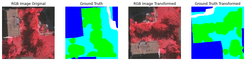
Original training patch with its ground truth mask.
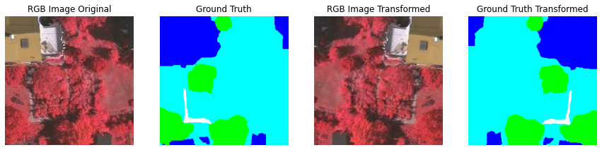
The same patch after random augmentation — note how both the image and mask are transformed consistently.
3. DeepLabV3+ Architecture
DeepLabV3+ represents a fundamentally different approach to segmentation compared to U-Net. Instead of learning the entire feature hierarchy from scratch, it leverages a pre-trained ResNet50 backbone and introduces Atrous Spatial Pyramid Pooling (ASPP) to capture multi-scale context.
Key Components
- ResNet50 backbone — Pre-trained on ImageNet, providing rich feature representations from the start
- ASPP module — Applies parallel atrous (dilated) convolutions at rates 1, 6, 12, and 18, capturing context at multiple spatial scales without losing resolution
- Encoder-decoder with low-level feature fusion — Upsampled ASPP features are concatenated with low-level backbone features for precise boundary recovery
def DilatedSpatialPyramidPooling(dspp_input):
    dims = dspp_input.shape
    # Global average pooling branch
    x = AveragePooling2D(pool_size=(dims[-3], dims[-2]))(dspp_input)
    x = conv_bn_block(x, kernel_size=1, use_bias=True)
    out_pool = UpSampling2D(
        size=(dims[-3] // x.shape[1], dims[-2] // x.shape[2]),
        interpolation="bilinear")(x)
    # Atrous convolutions at different rates
    out_1 = conv_bn_block(dspp_input, kernel_size=1, dilation_rate=1)
    out_6 = conv_bn_block(dspp_input, kernel_size=3, dilation_rate=6)
    out_12 = conv_bn_block(dspp_input, kernel_size=3, dilation_rate=12)
    out_18 = conv_bn_block(dspp_input, kernel_size=3, dilation_rate=18)
    # Concatenate all branches
    x = Concatenate(axis=-1)([out_pool, out_1, out_6, out_12, out_18])
    return conv_bn_block(x, kernel_size=1)
The full DeepLabV3+ model extracts features at two levels from the ResNet50 backbone, applies ASPP to the deeper features, then upsamples and fuses with the shallower features:
def get_deeplabv3plus(img_size, n_classes):
    model_input = keras.Input(shape=(img_size, img_size, 3))
    resnet50 = ResNet50(weights="imagenet", include_top=False,
                        input_tensor=model_input)
    # Deep features from conv4_block6
    x = resnet50.get_layer("conv4_block6_2_relu").output
    x = DilatedSpatialPyramidPooling(x)
    # Upsample 4x
    input_a = UpSampling2D(size=(img_size // 4 // x.shape[1],
                                  img_size // 4 // x.shape[2]),
                           interpolation="bilinear")(x)
    # Low-level features from conv2_block3
    input_b = resnet50.get_layer("conv2_block3_2_relu").output
    input_b = conv_bn_block(input_b, num_filters=48, kernel_size=1)
    # Fuse deep + low-level features
    x = Concatenate(axis=-1)([input_a, input_b])
    x = conv_bn_block(x)
    x = conv_bn_block(x)
    # Final upsampling to original resolution
    x = UpSampling2D(size=(img_size // x.shape[1],
                           img_size // x.shape[2]),
                     interpolation="bilinear")(x)
    output = Conv2D(n_classes, kernel_size=1,
                    padding="same", activation="softmax")(x)
    return Model(inputs=model_input, outputs=output,
                 name="DeepLabV3Plus")
The DeepLabV3+ architecture built on ResNet50, showing the ASPP module, low-level feature fusion, and progressive upsampling.
4. Focal Loss for Class Imbalance
Standard categorical cross-entropy treats all pixels equally, but the Vaihingen dataset is heavily imbalanced — classes like "car" and "clutter" occupy far fewer pixels than "tree" or "building." Focal loss addresses this by down-weighting well-classified examples and focusing the model's attention on hard, misclassified pixels:
Lfocal(pt) = −α(1 − pt)γ log(pt)
- α (alpha = 0.25) — A weighting factor that balances the importance of different classes
- γ (gamma = 2.0) — A focusing parameter that reduces the loss contribution from easy examples. When γ = 0, focal loss reduces to standard cross-entropy
def categorical_focal_loss(gamma=2.0, alpha=0.25):
    def focal_loss(y_true, y_pred):
        epsilon = K.epsilon()
        y_pred = K.clip(y_pred, epsilon, 1.0 - epsilon)
        cross_entropy = -y_true * K.log(y_pred)
        weight = alpha * y_true * K.pow((1 - y_pred), gamma)
        loss = weight * cross_entropy
        return K.mean(K.sum(loss, axis=-1))
    return focal_loss
5. Experimental Comparison
We train four model configurations to isolate the effect of each improvement:
- U-Net — Baseline without augmentation
- U-Net + Augmentation — Same architecture with data augmentation
- DeepLabV3+ + Augmentation — ResNet50 backbone with augmentation and cross-entropy loss
- DeepLabV3+ + Augmentation + Focal Loss — Same as above but with focal loss
# All four models trained with:
epochs = 200
batch_size = 8
patch_size = 256
# ModelCheckpoint monitoring val_iou, EarlyStopping patience=30
Results
| Model | Train Acc | Train IoU | Val IoU | Test Acc | Test IoU |
|---|---|---|---|---|---|
| U-Net | 78.54% | 0.509 | 0.468 | 76.30% | 0.454 |
| U-Net + Aug | 83.33% | 0.601 | 0.529 | 79.62% | 0.512 |
| DeepLabV3+ + Aug | 93.15% | 0.792 | 0.604 | 84.96% | 0.643 |
| DeepLabV3+ + Aug + Focal | 92.22% | 0.779 | 0.590 | 84.73% | 0.636 |
Key observations:
- Data augmentation consistently helps. Adding augmentation to U-Net improves test IoU from 0.454 to 0.512 (+12.8% relative improvement).
- DeepLabV3+ significantly outperforms U-Net. The ResNet50 backbone with ASPP achieves 0.643 test IoU vs U-Net's 0.512, a 25.6% relative improvement. The pre-trained backbone provides a strong feature initialization that U-Net (trained from scratch) cannot match.
- Focal loss provides marginal benefit here. The difference between cross-entropy (0.643) and focal loss (0.636) is small, suggesting that the class imbalance effect is partially mitigated by the augmentation and the model's capacity.
6. Prediction Visualizations
Comparing predictions from all four models on the same test patches reveals the progressive improvement in segmentation quality:

Prediction comparison: RGB input, ground truth, and outputs from all four models with per-class IoU scores. DeepLabV3+ produces notably sharper boundaries.

Another test patch comparison. The DeepLabV3+ models capture finer structural details, particularly along building edges and road boundaries.
7. Key Takeaways
- Pre-trained backbones are a game changer. DeepLabV3+ with ResNet50 (pre-trained on ImageNet) dramatically outperforms U-Net trained from scratch, even though ImageNet contains natural images rather than aerial imagery. Transfer learning provides a strong feature initialization.
- Atrous convolutions capture multi-scale context. ASPP applies dilated convolutions at rates 1, 6, 12, and 18, enabling the model to simultaneously consider local details and broader spatial context without losing resolution.
- Data augmentation is a low-cost, high-impact improvement. Simple geometric transforms (flips, rotations, shifts) applied consistently to both image and mask provide meaningful regularization, especially with limited training data.
- Focal loss is not always necessary. While theoretically sound for class imbalance, its benefit depends on the severity of imbalance and other regularization strategies already in use.
- Architecture matters more than loss function. The jump from U-Net to DeepLabV3+ (+25.6% IoU) far exceeds the effect of switching loss functions (−1.1% IoU), underscoring the importance of architectural design choices.
Moving from U-Net to DeepLabV3+ is not merely swapping architectures — it is embracing pre-trained representations, multi-scale reasoning, and efficient upsampling. These principles extend beyond segmentation to any dense prediction task in remote sensing.